Support Vector Machine (SVM) Algorithm – Machine Learning | Everything You Need to Know

Last updated on 29th Dec 2021, Blog, General

(5.0) | 19568 Ratings 1738

Share:

Support Vector Machine” (SVM) is a supervised machine learning algorithm that can be used for both classification or regression challenges. Support Vectors are simply the coordinates of individual observation. The SVM classifier is a frontier that best segregates the two classes (hyper-plane/ line).

• Introduction to Support Vector Machine
• Motivation
• Definition
• Application
• History
• Linear SVM
• Advantages and Disadvantages of SVM Classifier
• How an SVM works
• Why SVMs are used in machine learning
• Conclusion

Introduction to Support Vector Machine:

In machine learning, support-vector machines (SVMs, also support-vector networks [1]) are supervised learning models with associated learning algorithms that analyse data for classification and regression analysis. Developed at AT&T Bell Laboratories by Vladimir Vapnik with colleagues (Bosser et al., 1992; Gion et al., 1993; Cortés and Vapnik, 1995, [2] Vapnik et al., 1997 [citation needed]) SVMs include these. are one of The most robust prediction methods based on the statistical learning framework, or VC theory, proposed by Wapnik (1982, 1995) and Chervonenkis (1974).




Given a set of training examples, each marked as one of two categories, an SVM training algorithm builds a model that assigns new examples to one category or the other, making it a non-probability Becomes a binary linear classifier (although methods such as Platt scaling exist for using SVMs in a probabilistic classification setting). SVM maps training examples to points in space so as to maximise the width of the gap between the two categories. The new examples are then mapped to the same space and inferred as to which category they belong to, based on which side of the interval they fall.




In addition to performing linear classification, SVMs can efficiently perform a non-linear classification called the kernel trick, which maps their inputs to a higher-dimensional feature space indirectly. When the data is unlabeled, supervised learning is not possible, and a non-supervised learning approach is needed, which attempts to find the natural clustering of the data for the clusters, and then the clustering of these formed clusters. Maps new data to The support-vector clustering[3] algorithm, created by Hawa Siegelman and Vladimir Vapnik, applies data to support vectors developed in the Support Vector Machine algorithm to classify unlabeled data.

Motivation:

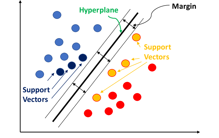
Classifying data is a common task in machine learning. Suppose some given data point each belongs to one of two classes, and the goal is to decide which class a new data point will belong to. In the case of support-vector machines, the data point is seen as p-dimensional vector ({\displaystyle p}p a list of numbers), and we want to know whether we can distinguish such points from a {\displaystyle (p-1)}(p-1)-dimensional hyperplane.




This is called a linear classifier. There are many hyperplanes that can classify data. A reasonable choice as to the best hyperplane is the one that represents the greatest separation or margin between two classes. So we choose the hyperplane so that the distance from each side to the nearest data point is maximum. If such a hyperplane exists, it is known as a maximum-margin hyperplane and the linear classifier defined by it is known as a maximum-margin classifier; Or equivalently, the perceptron of optimum stability.

Definition:

More formally, a support-vector machine constructs a hyperplane or set of hyperplanes in a higher or infinite-dimensional space, which can be used for classification, regression, or other tasks such as outlier detection. [4] Intuitively, a good separation is achieved by the hyperplane that has the greatest distance to the training-data point closest to any class (the so-called functional margin), because in general the larger the margin, the greater the distance of the classifier. The normalisation error is low.




kernel machine:

• While the original problem can be stated in a finite-dimensional space, it is often the case that the discriminant sets are not linearly separable in that space. For this reason, it was proposed [6] that the original finite-dimensional space be mapped to a much higher-dimensional space, possibly to ease the separation in that space.


• To keep the computational load reasonable, the mappings used by SVM schemes are designed to ensure that the dot products of pairs of input data vectors can be easily computed in terms of variables in the original space, They have been chosen to correspond to the problem {\displaystyle k(x,y)}{\displaystyle k(x,y)} whose dot product is constant with a vector in that space, where such a set of vectors is an orthogonal (and thus minimal) set of vectors that defines the hyperplane.


• The vectors defining the hyperplane can be chosen as a linear combination with the parameter {\displaystyle \alpha _{i}}\alpha _{i} of the images of the feature vectors {\displaystyle x_{i}}x_{ i} which are in the database. With this hyperplane option, the point in the feature space mapped to the hyperplane is defined by the relation {\displaystyle \textstyle \sum _{i}\alpha _{i}k(x_ { i},x)={\text{constant}}.}{\displaystyle \textstyle \sum _{i}\alpha _{i}k( x_{i},x)={\text{constant}} . }


• Note that if proceeding from {\displaystyle k(x,y)}{\displaystyle k(x,y)} {\displaystyle y}y {\displaystyle y}y, {\displaystyle x}x The sum gets smaller as each term. Measures the degree of proximity of the test point {\displaystyle x}the corresponding data base point {\displaystyle x_{i}}x_{i} In this way, the sum of the above kernels can be used to measure the relative proximity of each test point to discriminate data points originating in one or the other set. Note the fact that the set of points mapped to any hyperplane {\displaystyle x}x can be quite complex as a result, allowing more complex differentiation between sets that are absolutely in the original space. are not convex. x_{i},x)={\text{constant}}

Application:

SVMs can be used to solve various real-world problems: SVMs are helpful in text and hypertext classification, as their application can significantly reduce the need for label training examples in both standard inductive and transductive settings. [8] Some methods for shallow semantic parsing are based on support vector machines.




Images can also be classified using SVM. Experimental results show that SVMs achieve significantly higher search accuracy than traditional query refinement schemes after only three to four rounds of contextual feedback. This is also true for image partitioning systems, including systems using modified version SVMs that use the privileged approach suggested by wapnik.



• Classification of satellite data such as SAR data using supervised SVM.
• Handwritten characters can be recognized using SVM.
• The SVM algorithm has been widely applied in biological and other sciences.
• They have been used to classify proteins correctly for up to 90% of compounds.
• Permutation tests based on SVM weights have been suggested as a mechanism for interpreting SVM models.
• Support-vector machine weights have also been used to interpret SVM models in the past.
• Post Hoc interpretation of support-vector machine models to identify features used by models to make predictions is a relatively new area of research with particular importance in the biological sciences.

History:

The original SVM algorithm was invented by Vladimir N. Vapnik and Alexey Yes did. Chervonenkis in 1963. In 1992, Bernhard Bowser, Isabel Gyön, and Vladimir Vapnik suggested a way to create nonlinear classifiers by applying the kernel trick to a maximum-margin hyperplane. The “soft margin” embodiment, as in commonly used software packages, was proposed by Corinna Cortés and Vapnik in 1993 and published in 1995.

Linear SVM:

Svm kernel

In practice, the SVM algorithm is implemented with a kernel that transforms an input data space as needed. SVM uses a technique called kernel trick in which the kernel takes a low dimensional input space and transforms it into a higher dimensional space. In simple words, the kernel converts non-separable problems into separable problems by adding more dimensions. This makes SVM more powerful, flexible and accurate. Following are some types of kernels used by SVM.




Linear kernel

• It can be used as the dot product between any two observations. The formula of linear kernel is given below –
• k(x, xi) = sum(x∗xi)
• From the above formula, we can see that the product between the two vectors and the sum of the product of each pair of input values.



Polynomial kernel

• It is a more generalised form of the linear kernel and differentiates curved or non-linear input space. Following is the formula for the polynomial kernel –
• k(X,Xi)=1+sum(X∗Xi)^d
• Here d is the degree of the polynomial, which we need to specify manually in the learning algorithm.



Radial Basis Function (RBF) Kernel

• The RBF kernel, mostly used in SVM classification, maps the input space to an indefinite dimensional space. The following formula explains it mathematically –
• K(x,xi)=exp(−gamma∗sum(x−xi^2))
• Here, the gamma ranges from 0 to 1. We need to specify it manually in the learning algorithm. A good default value of gamma is 0.1.

As we have implemented SVM for linearly separable data, we can implement it in Python for data which is not linearly separable. This can be done using kernels. Following is an example to create an SVM classifier using kernel. We scikit-learn − . will use the iris dataset from




Example:

We will start by importing the following packages –

• PD. import pandas as
• np. import numpy as
• sklearn import svm, from dataset
• plt. import matplotlib.pyplot as
• Now, we need to load the input data –
• iris = dataset. load_iris()
• From this dataset, we are taking the first two features as follows –
• x = iris.data [:, :2]
• y = iris.target
• Next, we will plot the SVM boundaries with the original data as follows –
• x_min, x_max = X[:, 0].min() – 1, X[:, 0].max() + 1
• y_min, y_max = X[:, 1].min() – 1, X[:, 1].max() + 1
• H = (x_max / x_min) / 100
• **, yy = np.meshgrid(np.arange(x_min, x_max, h), np.arange(y_min, y_max, h))
• X_plot = np.c_[**.ravel(), yy.ravel()]
• Now, we need to provide the value of the regularisation parameter as follows –
• c = 1.0
• After this, the SVM classifier object can be created as follows –
• svc_classifier = svm.SVC(kernel = ‘linear’, c = c). fit(x, y)
• Z = svc_classifier.predict(X_plot)
• Z = Z.reshape(**.size)
• plt.figure(fig =(15, 5))
• plt.subplot(121)
• plt.contourf(**, yy, Z, cmap=plt.cm.tab10, alpha=0.3)
• plt.scatter(X[:, 0], X[:, 1], c=y, cmap=plt.cm.Set1)
• plt.xlabel(‘sepal length’)
• plt.ylabel(‘sepal width’)
• plt.xlim(**.min(), **.max())
• plt.title(‘Support vector classifiers with linear kernel’)
• production
• text(0.5, 1.0, ‘Support vector classifier with linear’)

Advantages and Disadvantages of SVM Classifier:

Pros of SVM Classifier

SVM classifier provides high accuracy and works well with high dimensional space. SVM classifiers basically use a subset of the training points so the result uses very little memory.




Develop Your Skills with Advanced Machine Learning Certification Training
Weekday / Weekend BatchesSee Batch Details

Cons of SVM Classifier

They have high training time so in practice not suitable for large datasets. Another disadvantage is that the SVM classifier does not work well with overlapping classes.

How an SVM works:

A simple linear SVM classifier works by creating a straight line between two classes. This means that all the data points on one side of the line will represent one category and the data points on the other side of the line will be placed in a different category. This means that there can be an infinite number of lines to choose from.




What makes the linear SVM algorithm better than some other algorithms, such as k-nearest neighbours, is that it picks the best line to classify your data points. It chooses the line that separates the data and is as far from the closest data points as possible.




A 2-D example helps to understand all the machine learning jargon. Basically you have some data points on a grid. You’re trying to separate these data points by the range they should fit into, but you don’t want to put any data in the wrong category. This means that you are trying to find the line between two closest points that separates the other data points.




So the two closest data points give you the support vectors used to find that line. That line is called the decision boundary. The decision boundary does not have to be a line. It is also known as a hyperplane because you can find decision boundaries with many features, not just two.

Why SVMs are used in machine learning:

SVMs are used in applications such as handwriting recognition, intrusion detection, face detection, email classification, gene classification and web pages. This is one of the reasons why we use SVMs in machine learning. It can handle both classification and regression on linear and non-linear data.

Another reason we use SVMs is because they can find complex relationships between your data without requiring you to do a lot of transformations on your own. This is a great option when you are working with small datasets that contain tens to hundreds of thousands of features. They generally yield more accurate results than other algorithms due to their ability to handle small, complex datasets.




Here are some advantages and disadvantages of using SVM:

• Professionals
• Effective on datasets with multiple characteristics, such as financial or medical data.
• Effective in cases where the number of features exceeds the number of data points.
• Uses a subset of training points in the decision function called support vectors to make it memory efficient.
• Various kernel functions can be specified for the decision function. You can use the normal kernel, but it is also possible to specify a custom kernel.
• Shortcoming
• If the number of features is much higher than the number of data points, it is important to avoid overfitting when choosing kernel functions and regularisation terms.
• SVMs do not directly provide probability estimates. They are calculated using an expensive five-fold cross-validation.
• Works best on small sample sets due to its high training time.
• Since SVMs can use any number of kernels, it is important that you are aware of some of them.

Conclusion:

• A support vector machine is a machine learning model capable of generalising between two different classes if a set of labelled data is provided in the training set of the algorithm. The main function of SVM is to check the hyperplane that is capable of distinguishing between two classes.


• There may be many hyperplanes which can perform this task but the objective is to find the hyperplane which has the greatest margin i.e. the maximum distance between two classes, so that in future if a new data point comes which is two then it is called Can be classified can be classified easily.


• In this blog, I have tried to explain to you about the Support Vector Machine and how it works. I have talked about linearly as well as non linearly separable data, also discussed kernel tricks, kernel functions and degree of tolerance in SVM. Finally I talked about the pros and cons of Support Vector Machine followed by a description of the problem on the cancer dataset.