PySpark MLlib-Tutorial – Best Resources To Learn in 1 Day | CHECK OUT

Last updated on 10th Jul 2020, Blog, Tutorials

Spark 

Apache Spark is a lightning fast real-time processing framework. It does in-memory computations to analyze data in real-time. It came into picture as Apache Hadoop MapReduce was performing batch processing only and lacked a real-time processing feature. Hence, Apache Spark was introduced as it can perform stream processing in real-time and can also take care of batch processing.

Apart from real-time and batch processing, Apache Spark supports interactive queries and iterative algorithms also. Apache Spark has its own cluster manager, where it can host its application. It leverages Apache Hadoop for both storage and processing. It uses HDFS (Hadoop Distributed File system) for storage and it can run Spark applications on YARN as well.

PySpark 

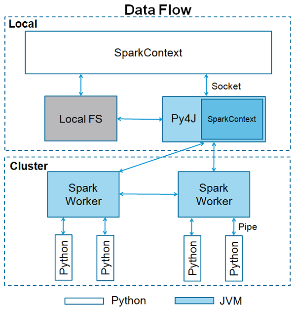
Apache Spark is written in the Scala programming language. To support Python with Spark, Apache Spark Community released a tool, PySpark. Using PySpark, you can work with RDDs in Python programming language also. It is because of a library called Py4j that they are able to achieve this.

PySpark offers PySpark Shell which links the Python API to the spark core and initializes the Spark context. Majority of data scientists and analytics experts today use Python because of its rich library set. Integrating Python with Spark is a boon to them.

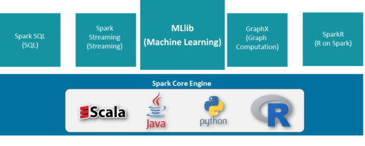
Apache Spark offers a Machine Learning API called MLlib. PySpark has this machine learning API in Python as well. It supports different kind of algorithms, which are mentioned below.

• mllib.classification 

The spark.mllib package supports various methods for binary classification, multiclass classification and regression analysis. Some of the most popular algorithms in classification are Random Forest, Naive Bayes, Decision Tree, etc.

•  mllib.clustering 

Clustering is an unsupervised learning problem, whereby you aim to group subsets of entities with one another based on some notion of similarity.

• mllib.fpm 

 Frequent pattern matching is mining frequent items, itemsets, subsequences or other substructures that are usually among the first steps to analyze a large-scale dataset. This has been an active research topic in data mining for years.

• mllib.linalg 

MLlib utilities for linear algebra.

• mllib.recommendation 

Collaborative filtering is commonly used for recommender systems. These techniques aim to fill in the missing entries of a user item association matrix.

• spark.mllib 

It ¬currently supports model-based collaborative filtering, in which users and products are described by a small set of latent factors that can be used to predict missing entries. spark.mllib uses the Alternating Least Squares (ALS) algorithm to learn these latent factors.

• mllib.regression 

 Linear regression belongs to the family of regression algorithms. The goal of regression is to find relationships and dependencies between variables. The interface for working with linear regression models and model summaries is similar to the logistic regression case.

There are other algorithms, classes and functions also as a part of the mllib package. As of now, let us understand a demonstration on pyspark.mllib.

SparkContext 

SparkContext is the entry point to any spark functionality. When we run any Spark application, a driver program starts, which has the main function and your SparkContext gets initiated here. The driver program then runs the operations inside the executors on worker nodes.

SparkContext uses Py4J to launch a JVM and creates a JavaSparkContext. By default, PySpark has SparkContext available as ‘sc’, so creating a new SparkContext won’t work.

Parameters

Following are the parameters of a SparkContext.

• Master  

It is the URL of the cluster it connects to.

• appName 

Name of your job.

• sparkHome 

Spark installation directory.

• pyFiles 

The .zip or .py files to send to the cluster and add to the PYTHONPATH.

• Environment 

Worker nodes environment variables.

• batchSize 

The number of Python objects represented as a single Java object. Set 1 to disable batching, 0 to automatically choose the batch size based on object sizes, or -1 to use an unlimited batch size.

• Serializer 

RDD serializer.

• Conf 

An object of L{SparkConf} to set all the Spark properties.

• Gateway 

Use an existing gateway and JVM, otherwise initializing a new JVM.

• JSC 

The JavaSparkContext instance.

• profiler_cls 

A class of custom Profiler used to do profiling (the default is pyspark.profiler.BasicProfiler).

MLlib – Classification and Regression

MLlib supports various methods for binary classification, multiclass classification, and regression analysis. The table below outlines the supported algorithms for each type of problem.

• linear models (SVMs, logistic regression, linear regression)
• naive Bayes
• decision trees
• ensembles of trees (Random Forests and Gradient-Boosted Trees)

MLlib – Linear Methods

Mathematical formulation

• Loss functions
• Regularizes
• Optimization
• Binary classification
• Linear Support Vector Machines (SVMs)
• Logistic regression
• Evaluation metrics
• Linear least squares, Lasso, and ridge regression
• Streaming linear regression

Mathematical formulation

Many standard machine learning methods can be formulated as a convex optimization problem, i.e. the task of finding a minimizer of a convex function ff that depends on a variable vector ww (called weights in the code), which has dd entries. Formally, we can write this as the optimization problem

Loss functions

The following table summarizes the loss functions and their gradients or sub-gradients for the methods MLlib supports:

Regularizers

The purpose of the regularize is to encourage simple models and avoid over-fitting. We support the following regularizes in MLlib:

Optimization

Under the hood, linear methods use convex optimization methods to optimize the objective functions. MLlib uses two methods, SGD and L-BFGS, described in the optimization section. Currently, most algorithm APIs support Stochastic Gradient Descent (SGD), and a few support L-BFGS. Refer to this optimization section for guidelines on choosing between optimization methods.

Binary classification

Binary classification aims to divide items into two categories: positive and negative. MLlib supports two linear methods for binary classification: linear Support Vector Machines (SVMs) and logistic regression. For both methods, MLlib supports L1 and L2 regularized variants. The training data set is represented by an RDD of LabeledPoint in MLlib. Note that, in the mathematical formulation in this guide, a training label yy is denoted as either +1+1 (positive) or −1−1 (negative), which is convenient for the formulation. However, the negative label is represented by 00 in MLlib instead of −1−1, to be consistent with multiclass labeling.

Linear Support Vector Machines (SVMs)

The linear SVM is a standard method for large-scale classification tasks. It is a linear method as described above in equation (1), with the loss function in the formulation given by the hinge loss:

L(w;x,y):=max{0,1−ywTx}.L(w;x,y):=max{0,1−ywTx}.

By default, linear SVMs are trained with an L2 regularization. We also support alternative L1 regularization. In this case, the problem becomes a linear program.

The linear SVMs algorithm outputs an SVM model. Given a new data point, denoted by xx, the model makes predictions based on the value of wTx Tx. By the default, if wTx≥0wTx≥0 then the outcome is positive, and negative otherwise.

Logistic regression

Logistic regression is widely used to predict a binary response. It is a linear method as described above in equation (1), with the loss function in the formulation given by the logistic loss:

L(w;x,y):=log(1+exp(−ywTx)).L(w;x,y):=log⁡(1+exp⁡(−ywTx)).

The logistic regression algorithm outputs a logistic regression model. Given a new data point, denoted by xx, the model makes predictions by applying the logistic function

f(z)=11+e−zf(z)=11+e−z

where z=wTxz=wTx. By default, if f(wTx)>0.5f(wTx)>0.5, the outcome is positive, or negative otherwise, though unlike linear SVMs, the raw output of the logistic regression model, f(z)f(z), has a probabilistic interpretation (i.e., the probability that xx is positive).

Evaluation metrics

MLlib supports common evaluation metrics for binary classification (not available in PySpark). This includes precision, recall, F-measure, receiver operating characteristic (ROC), precision-recall curve, and area under the curves (AUC). AUC is commonly used to compare the performance of various models while precision/recall/F-measure can help determine the appropriate threshold to use for prediction purposes.

The following code snippet illustrates how to load a sample dataset, execute a training algorithm on this training data using a static method in the algorithm object, and make predictions with the resulting model to compute the training error.

The SVM With SGD.train() method by default performs L2 regularization with the regularization parameter set to 1.0. If we want to configure this algorithm, we can customize SVM With SGD further by creating a new object directly and calling setter methods. All other MLlib algorithms support customization in this way as well. For example, the following code produces an L1 regularized variant of SVMs with regularization parameter set to 0.1, and runs the training algorithm for 200

Linear least squares, Lasso, and ridge regression

Linear least squares is the most common formulation for regression problems. It is a linear method as described above in equation (1), with the loss function in the formulation given by the squared loss:

Various related regression methods are derived by using different types of regularization: ordinary least squares or linear least squares uses no regularization; ridge regression uses L2 regularization; and Lasso uses L1 regularization. For all of these models, the average loss or training error, 1n∑ni=1(wTxi−yi)21n∑i=1n(wTxi−yi)2, is known as the mean squared error

JavaIn order to run the above application, follow the instructions provided in the Self-Contained Applications section of the Spark quick-start guide. Be sure to also include spark–mllib to your build file as a dependency.

Streaming linear regression

When data arrive in a streaming fashion, it is useful to fit regression models online, updating the parameters of the model as new data arrives. MLlib currently supports streaming linear regression using ordinary least squares. The fitting is similar to that performed offline, except fitting occurs on each batch of data, so that the model continually updates to reflect the data from the stream.

MLlib – Naive Bayes

Naive Bayes is a simple multiclass classification algorithm with the assumption of independence between every pair of features. Naive Bayes can be trained very efficiently. Within a single pass to the training data, it computes the conditional probability distribution of each feature given label, and then it applies Bayes’ theorem to compute the conditional probability distribution of label given an observation and use it for prediction.

MLlib supports multinational naive Bayes, which is typically used for document classification. Within that context, each observation is a document and each feature represents a term whose value is the frequency of the term. Feature values must be non negative to represent term frequencies. Additive smoothing can be used by setting the parameter 

For document classification, the input feature vectors are usually sparse, and sparse vectors should be supplied as input to take advantage of sparsity. Since the training data is only used once, it is not necessary to cache it.

MLlib – Decision Tree

• Basic algorithm
• Node impurity and information gain
• Split candidates
• Stopping rule
• Usage tips
• Problem specification parameters
• Stopping criteria
• T unable parameters
• Caching and check pointing
• Scaling

Decision Trees

Decision trees and their ensembles are popular methods for the machine learning tasks of classification and regression. Decision trees are widely used since they are easy to interpret, handle categorical features, extend to the multi class classification setting, do not require feature scaling, and are able to capture non-literariness and feature interactions. Tree ensemble algorithms such as random forests and boosting are among the top performers for classification and regression tasks.

MLlib supports decision trees for binary and multiclass classification and for regression, using both continuous and categorical features. The implementation partitions data by rows, allowing distributed training with millions of instances.

Ensembles of trees (Random Forests and Gradient-Boosted Trees) are described in the Ensembles guide.

Basic algorithm

The decision tree is a greedy algorithm that performs a recursive binary partitioning of the feature space. The tree predicts the same label for each bottom most (leaf) partition. Each partition is chosen greedily by selecting the best split from a set of possible splits, in order to maximize the information gain at a tree node. In other words, the split chosen at each tree node is chosen from the set 

Node impurity and information gain

The node impurity is a measure of the homogeneity of the labels at the node. The current implementation provides two impurity measures for classification (Gini impurity and entropy) and one impurity measure for regression (variance).

Split candidates

Continuous features

For small datasets in single-machine implementations, the split candidates for each continuous feature are typically the unique values for the feature. Some implementations sort the feature values and then use the ordered unique values as split candidates for faster tree calculations.

Sorting feature values is expensive for large distributed datasets. This implementation computes an approximate set of split candidates by performing a quantile calculation over a sampled fraction of the data. The ordered splits create “bins” and the maximum number of such bins can be specified using the maxBins parameter.

Stopping rule

The recursive tree construction is stopped at a node when one of the following conditions is met:

• The node depth is equal to the maxDepth training parameter.
• No split candidate leads to an information gain greater than minInfoGain.
• No split candidate produces child nodes which each have at least minInstancesPerNode training instances.

Usage tips

We include a few guidelines for using decision trees by discussing the various parameters. The parameters are listed below roughly in order of descending importance. New users should mainly consider the “Problem specification parameters” section and the maxDepth parameter.

Problem specification parameters

These parameters describe the problem you want to solve and your dataset. They should be specified and do not require tuning.

• algo: Classification or Regression

• num Classes: Number of classes (for Classification only)

• categorical Features Info: Specifies which features are categorical and how many categorical values each of those features can take. This is given as a map from feature indices to feature arity (number of categories). Any features not in this map are treated as continuous.

• E.g., Map(0 -> 2, 4 -> 10) specifies that feature 0 is binary (taking values 0 or 1) and that feature 4 has 10 categories (values {0, 1, …, 9}). Note that feature indices are 0-based: features 0 and 4 are the 1st and 5th elements of an instance’s feature vector.
• Note that you do not have to specify categoricalFeaturesInfo. The algorithm will still run and may get reasonable results. However, performance should be better if categorical features are properly designated.

Stopping criteria

These parameters determine when the tree stops building (adding new nodes). When tuning these parameters, be careful to validate on held-out test data to avoid overfitting.

• maxDepth: Maximum depth of a tree. Deeper trees are more expressive (potentially allowing higher accuracy), but they are also more costly to train and are more likely to overfit.
• minInstancesPerNode: For a node to be split further, each of its children must receive at least this number of training instances. This is commonly used with RandomForest since those are often trained deeper than individual trees.
• minInfoGain: For a node to be split further, the split must improve at least this much (in terms of information gain).

Tunable parameters

These parameters may be tuned. Be careful to validate on held-out test data when tuning in order to avoid overfitting.

• maxBins: Number of bins used when discretizing continuous features.

• Increasing maxBins allows the algorithm to consider more split candidates and make fine-grained split decisions. However, it also increases computation and communication.
• Note that the maxBins parameter must be at least the maximum number of categories 
• M for any categorical feature.
• maxMemoryInMB: Amount of memory to be used for collecting sufficient statistics.The default value is conservatively chosen to be 256 MB to allow the decision algorithm to work in most scenarios. Increasing maxMemoryInMB can lead to faster training (if the memory is available) by allowing fewer passes over the data. However, there may be decreasing returns as maxMemoryInMB grows since the amount of communication on each iteration can be proportional to maxMemoryInMB.
• Implementation details: For faster processing, the decision tree algorithm collects statistics about groups of nodes to split (rather than 1 node at a time). The number of nodes which can be handled in one group is determined by the memory requirements (which vary per features). The maxMemory in MB parameter specifies the memory limit in terms of megabytes which each worker can use for these statistics.
• subsampling Rate: Fraction of the training data used for learning the decision tree. This parameter is most relevant for training ensembles of trees (using Random Forest and Gradient Boosted Trees), where it can be useful to sub sample the original data. For training a single decision tree, this parameter is less useful since the number of training instances is generally not the main constraint.

• impurity: Impurity measure (discussed above) used to choose between candidate splits. This measure must match the algo parameter.

• Caching and check pointing : MLlib 1.2 adds several features for scaling up to larger (deeper) trees and tree ensembles. When maxDepth is set to be large, it can be useful to turn on node ID caching and check pointing. These parameters are also useful for Random Forest when num trees is set to be large.

• use NodeId Cache: If this is set to true, the algorithm will avoid passing the current model (tree or trees) to executors on each iteration.This can be useful with deep trees (speeding up computation on workers) and for large Random Forests (reducing communication on each iteration).
• Implementation details: By default, the algorithm communicates the current model to executors so that executors can match training instances with tree nodes. When this setting is turned on, then the algorithm will instead cache this information.Node ID caching generates a sequence of RDDs (1 per iteration). This long lineage can cause performance problems, but check pointing intermediate RDDs can alleviate those problems. Note that check pointing is only applicable when use NodeIdCache is set to true.

• check point Dir: Directory for check pointing node ID cache RDDs.

• check point Interval: Frequency for check pointing node ID cache RDDs. Setting this too low will cause extra overhead from writing to HDFS; setting this too high can cause problems if executors fail and the RDD needs to be recomputed.

• Scaling : Computation scales approximately linearly in the number of training instances, in the number of features, and in the maxBins parameter. Communication scales approximately linearly in the number of features and in maxBins.The implemented algorithm reads both sparse and dense data. However, it is not optimized for sparse input.

Conclusion

Machine Learning denotes a step taken forward in how computers can learn and make predictions. It has applications in various sectors and is being extensively used. Having knowledge of Machine Learning will not only open multiple doors of opportunities for you, but it also makes sure that, if you have mastered Machine Learning, you are never out of jobs.

Machine Learning has been gaining popularity ever since it came into the picture and it won’t stop any time soon. So, without further ado, check out the Machine Learning Certification by ACTE and get started with Machine Learning today!