What is Logistic Regression? Explained with Examples

Introduction to Logistic Regression

Logistic Regression is one of the most widely used algorithms in statistical modeling and Machine Learning Training for binary classification problems. Despite the term “regression,” it is primarily used for classification tasks, such as determining whether a customer will purchase a product (yes or no), if an email is spam, or if a patient has a disease. Unlike linear regression, which predicts continuous values, logistic regression predicts the probability that a given input belongs to a certain class. This is made possible by the sigmoid function, which converts linear outputs into a range between 0 and 1. These probabilities can then be mapped to discrete classes. Logistic regression is highly interpretable, efficient to train, and works well on linearly separable datasets, making it a staple in predictive modeling.

Ready to Get Certified in Machine Learning? Explore the Program Now Machine Learning Online Training Offered By ACTE Right Now!

Difference Between Linear and Logistic Regression

Gradient Boosting is a machine learning technique used for both regression and classification tasks. It builds models in a stage-wise fashion and generalizes them by allowing optimization of an arbitrary differentiable loss function. Gradient Boosting is a type of boosting technique where new models are created to correct the errors made by previous models. Models are added sequentially, and each new model aims to reduce the residual errors of the combined ensemble of previous models. Unlike bagging, where models are built independently and then averaged, boosting builds models iteratively with each one focusing on fixing the mistakes of the previous ensemble. This sequential learning process makes gradient boosting highly effective in capturing complex patterns in data.

Subscribe To Contact Course Advisor

Subscribe

Sigmoid Function Explained

The sigmoid (or logistic) function transforms real-valued numbers into values between 0 and 1, which represent probabilities.

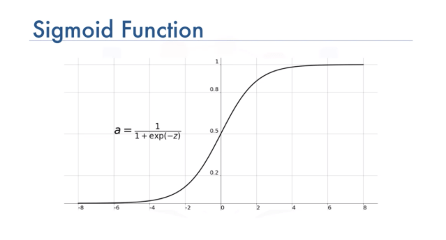
Formula:

• σ(z)=11+e−z\sigma(z) = \frac{1}{1 + e^{-z}}

Where zz is the linear combination of input features.

Properties:

• Output range: (0, 1)
• As z→∞z \rightarrow \infty, σ(z)→1\sigma(z) \rightarrow 1
• As z→−∞z \rightarrow -\infty, σ(z)→0\sigma(z) \rightarrow 0

This makes the sigmoid ideal for binary classification, as we can set a threshold (commonly 0.5) for decision making.

Binary Classification with Logistic Regression

In binary classification, logistic regression assigns the input to either class 0 or class 1 based on the computed probability.

Decision Rule:

• If P(y=1∣X)>0.5P(y=1|X) > 0.5, predict class 1.
• Else, predict class 0.

Loss Function:

The log loss (binary cross-entropy) is minimized during training:

• J(θ)=−1m∑i=1m[y(i)log⁡(hθ(x(i)))+(1−y(i))log⁡(1−hθ(x(i)))]J(\theta) = -\frac{1}{m} \sum_{i=1}^{m} \left[y^{(i)} \log(h_\theta(x^{(i)})) + (1 – y^{(i)}) \log(1 – h_\theta(x^{(i)}))\right]

Where hθ(x)h_\theta(x) is the output of the sigmoid function.

To Explore Machine Learning in Depth, Check Out Our Comprehensive Machine Learning Online Training To Gain Insights From Our Experts!

Assumptions and Conditions

For logistic regression to be effective, certain assumptions must hold true:

• Binary or Multiclass Dependent Variable
• Linearity in the Logit in the relationship between the independent variables and the log odds is linear.
• Independence of Observations
• No Multicollinearity among predictors
• Large Sample Size for stability

While logistic regression is robust, violation of these assumptions can lead to poor performance or biased predictions.

Model Training and Evaluation

Steps:

• Initialize: weights.
• Forward Pass: Compute sigmoid probabilities.
• Compute Loss: Use cross-entropy.
• Backpropagation: Compute gradients.
• Update Weights: using optimization (e.g., gradient descent).

Evaluation Metrics:

• Accuracy: (TP + TN) / Total
• Precision: TP / (TP + FP)
• Recall: TP / (TP + FN)
• F1 Score: Harmonic mean of precision and recall
• ROC-AUC: Evaluates classification across thresholds

Develop Your Skills with Machine Learning Training

Weekday / Weekend BatchesSee Batch Details

Implementation in Python

Here’s a simple example using scikit-learn:

• from sklearn.datasets import load_breast_cancer
• from sklearn.linear_model import LogisticRegression
• from sklearn.model_selection import train_test_split
• from sklearn.metrics import classification_report
• # Load data
• X, y = load_breast_cancer(return_X_y=True)
• # Split data
• X_train, X_test, y_train, y_test = train_test_split(X, y, test_size=0.3, random_state=42)
• # Train model
• model = LogisticRegression(max_iter=1000)
• model.fit(X_train, y_train)
• # Predict
• y_pred = model.predict(X_test)
• # Evaluate
• print(classification_report(y_test, y_pred))

Multiclass Logistic Regression

For problems with more than two classes, logistic regression is extended using:

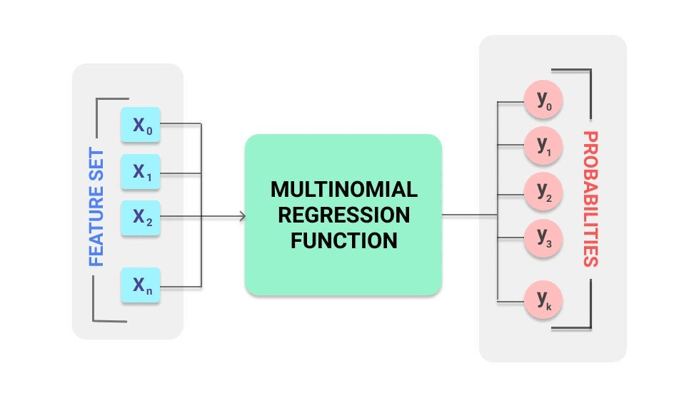
Techniques:

• One-vs-Rest (OvR): Trains one classifier per class.
• Multinomial Logistic Regression: Uses softmax to compute probabilities for each class.

Softmax Function:

• P(y=j)=ezj∑k=1KezkP(y = j) = \frac{e^{z_j}}{\sum_{k=1}^{K} e^{z_k}}

Scikit-learn supports both via:

LogisticRegression(multi_class=’multinomial’, solver=’lbfgs’)

Machine Learning Sample Resumes! Download & Edit, Get Noticed by Top Employers! Download

Advantages and Limitations

Advantages:

• Simple and easy to implement
• Interpretable model (especially for feature weights)
• Works well with linearly separable data
• Fast training

Limitations:

• Assumes linear decision boundary
• Poor performance with non-linear data
• Struggles with high-dimensional and highly correlated features
• Sensitive to outliers and noise

Applications (Healthcare, Marketing, etc.)

Logistic Regression is applied in multiple domains:

Healthcare:

• Predicting diseases (diabetes, cancer)
• Hospital readmission likelihood
• Risk assessment models

Marketing:

• Customer churn prediction
• Purchase intent detection
• Campaign response modeling

Finance:

• Credit scoring
• Loan default prediction
• Fraud detection

Web & Tech:

• Spam email detection
• Click-through rate (CTR) prediction
• User engagement analysis

Regularization Techniques

To combat overfitting, regularization is applied by adding a penalty to the loss function.

Types:

• L1 Regularization (Lasso): Promotes sparsity
• L2 Regularization (Ridge): Penalizes large weights

Updated Cost Function with L2:

• J(θ)=−log loss+λ∑j=1nθj2J(\theta) = -\text{log loss} + \lambda \sum_{j=1}^{n} \theta_j^2

Where λ\lambda is the regularization strength.

In Python:

LogisticRegression(penalty=’l2′, C=0.1)

Note: C is the inverse of regularization strength (lower C = more regularization).

Preparing for Machine Learning Job Interviews? Have a Look at Our Blog on Machine Learning Interview Questions and Answers To Ace Your Interview!

Summary and Insights

Logistic regression is a foundational classification algorithm that every data scientist must understand. It is not only a strong baseline but also a powerful model for linearly separable data with significant interpretability.

Key Takeaways:

• Converts linear models into probabilistic outputs using the sigmoid function.
• Highly efficient and interpretable for binary and multiclass problems.
• Evaluated using classification metrics like accuracy, F1 score, and AUC.
• Easily implemented using libraries like scikit-learn.
• Can be extended to handle multiple classes using softmax or OvR strategies.

As machine learning tasks grow more complex, understanding logistic regression helps lay a solid foundation for learning more advanced models like neural networks, decision trees, and ensemble methods.