Binomial Option Pricing Model | A step by step Guide

Last updated on 11th Jul 2020, Blog, General

The Binomial Option Pricing Model is a risk-neutral method for valuing path-dependent options (e.g., American options). It is a popular tool for stock options evaluation, and investors use the model to evaluate the right to buy or sell at specific prices over time.

Under this model, the current value of an option is equal to the present value of the probability-weighted future payoffs.

It is different from the Black-Scholes model, which is more suitable for path-independent options, which cannot be exercised before their due date.

Binomial Option Pricing Model

An investor knows the current stock price at any given moment. They will try to guess the stock price movements in the future. Under this model, we split the time to expiration of the option into equal periods (weeks, months, quarters). Then the model follows an iterative method to evaluate each period, considering either an up or down movement and the respective probabilities. Effectively, the model creates a binomial distribution of possible stock prices.

It’s mostly useful for American-style options, which investors can exercise at any given time. The model also assumes there’s no arbitrage, meaning there’s no buying while selling at a higher price. Having no-arbitrage ensures the value of the asset remains the same, which is a requirement for the Binomial Option Pricing model to work.

Assumptions

When setting up a binomial option pricing model, we need to be aware of the underlying assumptions, to understand the limitations of this approach better.

• At every point in time, the price can go to only two possible new prices, one up and one down (this is in the name, binomial);
• The underlying asset pays no dividends;
• The interest rate (discount factor) is a constant throughout the period;
• The market is frictionless, and there are no transaction costs and no taxes;
• Investors are risk-neutral, indifferent to risk;
• The risk-free rate remains constant.

Advantages and disadvantages

(+) The model is mathematically simple to calculate;

(+) Binomial Option Pricing is useful for American options, where the holder has the right to exercise at any time up until expiration.

(-) A significant advantage is a multi-period view the model provides for the underlying asset’s price and the transparency of the option’s value over time.

(-) A notable disadvantage is that the computational complexity rises a lot in multi-period models.

(-) The most significant limitation of the model is the inherent necessity to predict future prices.

How to Calculate the Model

If we set the current (spot) price of an option as S, then we can have two price movements at any given moment. The price can either go up to S+ or down to S-.

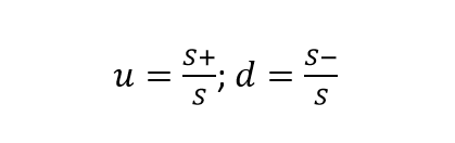
On this basis, we calculate the up(u) and down(d) factors.

Call Options

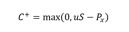
A call option entitles its holder to purchase the underlying asset or stock at the exercise price PX.

A call option is in-the-money when the spot price is above the exercise price (S > PX).

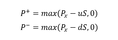
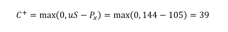
When we have an up movement, the payoff of the call option is the maximum between zero and the spot price multiplied by the up factor and reduced with the exercise price. To visualize that, here’s the formula

reduced with the exercise price. To visualize that, here’s the formula:

A downward movement gives a payoff of:

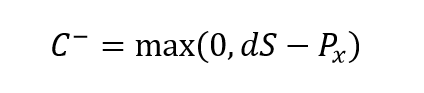
The Binomial model effectively weighs the different payoffs with their respective probabilities and discounts them to the present value.

Put Options

A put option entitles the holder to sell at the exercise price PX.

When the price goes down or up, we calculate a put option as follows:

Binomial Trees

The binomial tree is the best way to represent the model visually. They show the option payoff and probability at different nodes. Nodes outline the paths the price of the underlying asset may take over time.

We can represent a general one-period call option like this.

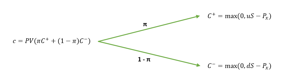
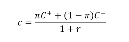
We can also present it as a formula:

The put option uses the same formula as the call option.

Where:

• π is the probability of an up move;
• r is the discount rate.

To arrive at the probability of an up move we employ the formula:

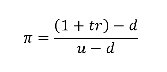
Where:

• t is the period multiplier (t = 0.5 for a 6-month period);
• r is the discount rate;
• d is the down factor
• u is the up factor.

In the case of a multi-period option, we can accumulate the additional stages by multiplying the up/down factors for every price movement. If we have an up move, followed by a down move, then we will udS in our formulas.

Binomial Tree Example

As an example, we can look at a call option with six months till maturity, and build a binomial tree with a period of three months.

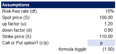
We will set the following assumptions:

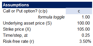
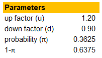
To set up our model, we need to calculate some parameters. We expect the price to either go up with 20% or down with 10% within a single time step. Applying the probability formula from above, we arrive at our model variables.

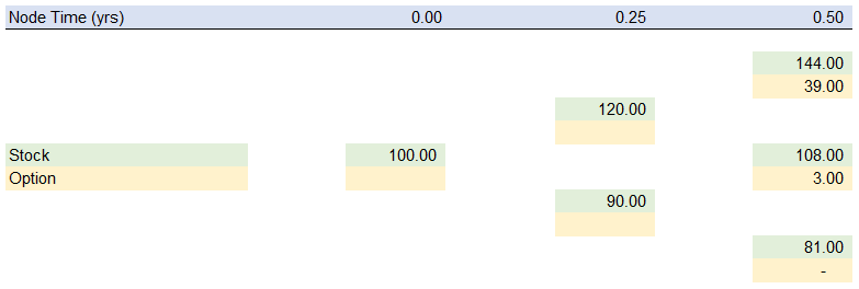
The next step is to construct the binomial tree for our model.

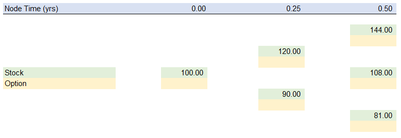
We set up the two time-steps for our period and end up with three positions in time — present, in three months and six months. Using the up and down factors, we can calculate the stock price at each of the nodes.

The next step is to calculate the option value at the terminal date (t=0.50). It equals the maximum of zero and the difference between the current price at t=0.50 and the strike price.

Working backward, we calculate the option value at t=0.25 and the present. We do this by weighing the possible future values with the up and down move probabilities and discounting them with the risk-free rate.

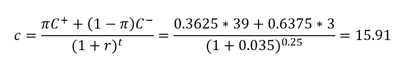
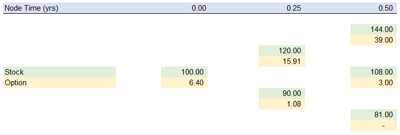
That way, we arrive at the present value of the option, at 6.40 euros.

Delta Portfolio Hedging

Delta Hedging is another approach to the binomial option pricing model. The idea is to build a synthetic hedge portfolio and find the profitability, at which the portfolio provides a risk-free payoff. That way, we can determine the trading value of the portfolio, and from there, the price of the option.

Here are the assumptions for our model:

The next step is to calculate the option payoff at the terminal date. We are looking at a one-period binomial model for the sake of simplicity, and our option value at period one will be.

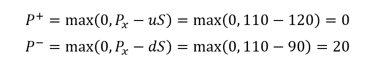
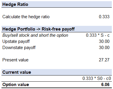
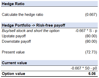
We can now use the option payoffs to calculate the Hedge Ratio, via the formula:

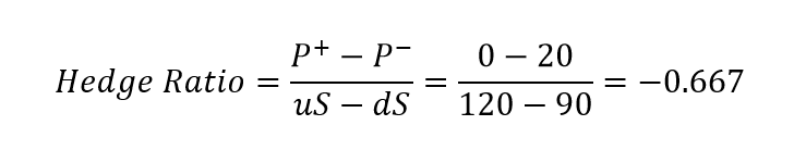
In reality, we will multiply the hedge ratio by some multiplier to make it a whole number, as we cannot typically trade in fractions of stocks. However, for this example, we will ignore that limitation of the real world.

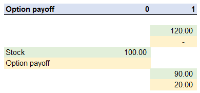
The next step is to build our portfolio. We will buy stock and then short the option. We calculate the portfolio value in the up and down states and expect these to be the same, because of the risk-free payoff assumption.

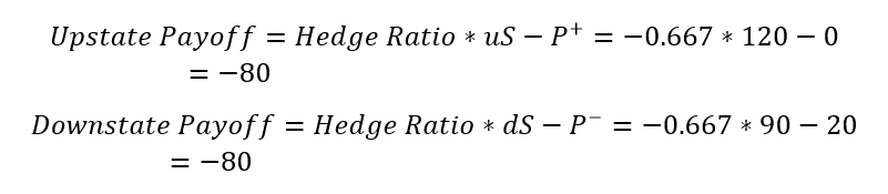
As our payoff is risk-free, this means the rate of return of the portfolio is the risk-free rate. Therefore the portfolio today should be worth the present value of the payoff. Using either of the up or down states, we can apply our risk-free discount factor of 10% and arrive at the current value of the payoff at -72.73.

If we adjust our portfolio function for the present we get:

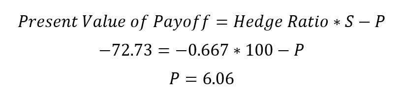
If we change only our assumption of the option type to a call, instead, we will get the same option value, due to the friction less market and no-arbitrage assumptions.