Object Detection Tensorflow: A Concise Tutorial Just An Hour – FREE

Last updated on 07th Jul 2020, Blog, Tutorials

What is object detection?

Given an image or a video stream, an object detection model can identify which of a known set of objects might be present and provide information about their positions within the image.For example, this screenshot of our example application shows how  objects have been recognized and their positions annotated:

Object detection

• Object detection is a computer vision technique that works to identify and locate objects within an image or video. Specifically, object detection draws bounding boxes around these detected objects, which allow us to locate where said objects are in (or how they move through) a given scene.
• Object detection is commonly confused with image recognition, so before we proceed, it’s important that we clarify the distinctions between them.
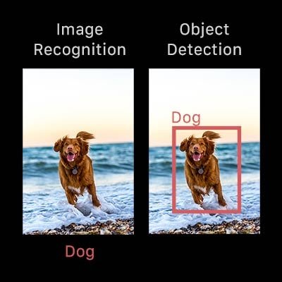
• Image recognition assigns a label to an image. A picture of a dog receives the label “dog”. A picture of two dogs still receives the label “dog”. Object detection, on the other hand, draws a box around each dog and labels the box “dog”. The model predicts where each object is and what label should be applied. In that way, object detection provides more information about an image than recognition.

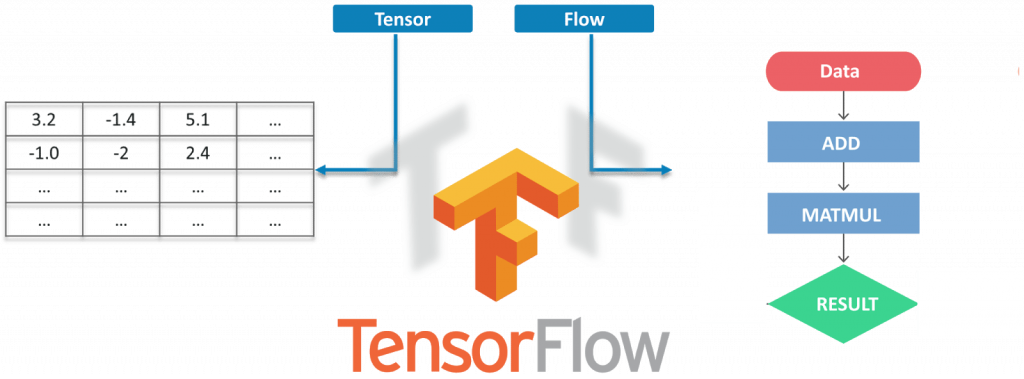
TensorFlow : Tensor flow is Google’s open-source machine learning framework for dataflow programming across a range of tasks. Nodes in the graph represent mathematical operations, while the graph edges represent the multidimensional data arrays (tensors) communicated between them.

Prerequisites :

Before working on the demo, let’s have a look at the prerequisites:

• Python
• TensorFlow
• TensorBoard
• Protobuf v3.4 or above
• Setting up the Environment

 To Download TensorFlow and TensorFlow GPU, you can use pip or conda commands:

For all the other libraries, we can use pip or conda to install them.

Next, we need to go inside the Tensorflow folder and then inside the research folder and run protobuf from there using this command:

“path_of_protobuf’s bin”./bin/protoc object_detection/protos/

To check whether this worked or not, you can go to the protos folder inside models>object_detection>protos and there, you can see that for every proto file, there’s one python file created.

Main Code :

• After the environment is set up, you need to go to the “object_detection” directory and create a new python file. You can use Spyder or Jupyter to write your code.
• First of all, we need to import all the libraries.

• Next, we will download the model, which is trained on the COCO dataset. COCO stands for Common Objects in Context, and this dataset contains around 330K labeled images. The model selection is important because you need to make a tradeoff between speed and accuracy. Depending on your requirement and the system memory, the correct model must be selected.
• “models>research>object_detection>g3doc>detection_model_zoo” contains all the models with different speed and accuracy (mAP).
• Next, we provide the required model and the frozen inference graph generated by Tensorflow.

This code will download that model from the internet and extract the frozen inference graph of that model.

Next, we are going to load all the labels

Now we will convert the images’ data into a NumPy array for processing.

The path to the images for the testing purpose is defined here. We have a naming convention “image[i]” for I in (1 to n+1), n being the number of images provided.

This code runs the inference for a single image where it detects the objects, make boxes, and provides the class and the class score of that particular object.

Our final loop, which will call all the functions defined above, will run the inference on all the input images one by one, which will provide us the output of images in which objects are detected with labels and the percentage/score of that object being similar to the training data.

Now, let’s see how we can detect objects in a live video feed.

Object Detection Using Tensorflow :

• For this demo, we will use the same code, but we’ll tweak a few things. We are going to use OpenCV and the camera module to use the live feed of the webcam to detect objects.
• Add the OpenCV library and the camera being used to capture images. Just add the following lines to the import library section.

We don’t need to load the images from the directory and convert it to NumPy array, as OpenCV will take care of that for us.

 Replace this:

With this:

We will not use matplotlib for the final image show. Instead, we will use OpenCV for that as well. For that.

Remove this:

This code will use OpenCV that will, in turn, use the camera object initialized earlier to open a new window named “Object_Detection” of the size “800×600”. It will wait for 25 milliseconds for the camera to show images, otherwise, it will close the window.

Final Code With All the Changes:

General object detection framework

Typically, there are three steps in an object detection framework.

1. First, a model or algorithm is used to generate regions of interest or region proposals. These region proposals are a large set of bounding boxes spanning the full image (that is, an object localisation component).
2. In the second step, visual features are extracted for each of the bounding boxes, they are evaluated and it is determined whether and which objects are present in the proposals based on visual features (i.e. an object classification component).
3. In the final post-processing step, overlapping boxes are combined into a single bounding box (that is, non maximum suppression).

Region proposals

Several different approaches exist to generate region proposals. Originally, the ‘selective search’ algorithm was used to generate object proposals. Lillie Weng provides a thorough explanation on this algorithm in her blog post. In short, selective search is a clustering based approach which attempts to group pixels and generate proposals based on the generated clusters.

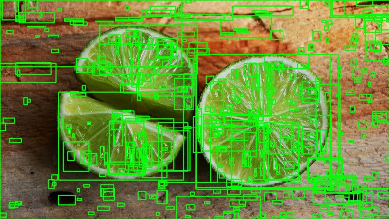
An example of a selective search applied to an image. A threshold can be tuned in the SS algorithm to generate more or fewer proposals.
Other approaches use more complex visual features extracted from the image to generate regions (for example, based on the features from a deep learning model) or adopt a brute-force approach to region generation. These brute-force approaches are similar to a sliding window that is applied to the image, over several ratios and scales. These regions are generated automatically, without taking into account the image features.

An example of the sliding window approach. Each of the bounding boxes will be used as a region of interest (ROI).
An important trade-off that is made with region proposal generation is the number of regions vs. the computational complexity. The more regions you generate, the more likely you will be able to find the object. On the flip-side, if you exhaustively generate all possible proposals, it won’t be possible to run the object detector in real-time, for example. In some cases, it is possible to use problem-specific information to reduce the number of ROIs. For example, pedestrians typically have a ratio of approximately 1.5, so it is not useful to generate ROI with a ratio of 0.25.

Feature extraction

The goal of feature extraction is to reduce a variable-sized image to a fixed set of visual features. Image classification models are typically constructed using strong visual feature extraction methods. Whether they are based on traditional computer vision approaches, such as for example, filter-based approached, histogram methods, etc., or deep learning methods, they all have the exact same objective: extract features from the input image that are representative for the task at hands and use these features to determine the class of the image. In object detection frameworks, people typically use pre-trained image classification models to extract visual features, as these tend to generalize fairly well. For example, a model trained on the MS CoCo dataset is able to extract fairly generic features. 

Non-maximum suppression

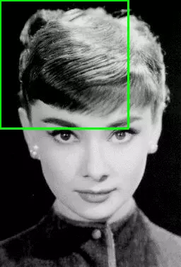
The general idea of non-maximum suppression is to reduce the number of detections in a frame to the actual number of objects present. If the object in the frame is fairly large and more than 2000 object proposals have been generated, it is quite likely that some of these will have significant overlap with each other and the object.NMS techniques are typically standard across the different detection frameworks, but it is an important step that might require hyperparameter tweaking based on the scenario.

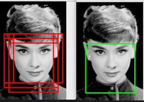
An example of NMS in the context of face detection.

Evaluation metric

The most common evaluation metric that is used in object recognition tasks is ‘mAP’, which stands for ‘mean average precision’. It is a number from 0 to 100 and higher values are typically better, but its value is different from the accuracy metric in classification.

Each bounding box will have a score associated (likelihood of the box containing an object). Based on the predictions a precision-recall curve (PR curve) is computed for each class by varying the score threshold. The average precision (AP) is the area under the PR curve. First, the AP is computed for each class and then averaged over the different classes. The end result is the mAP.

Note that detection is a true positive if it has an ‘intersection over union’ (IoU or overlap) with the ground-truth box greater than some threshold (usually 0.5). Instead of using mAP we typically use mAP@0.5 or mAP@0.25 to refer to the IoU that was used.

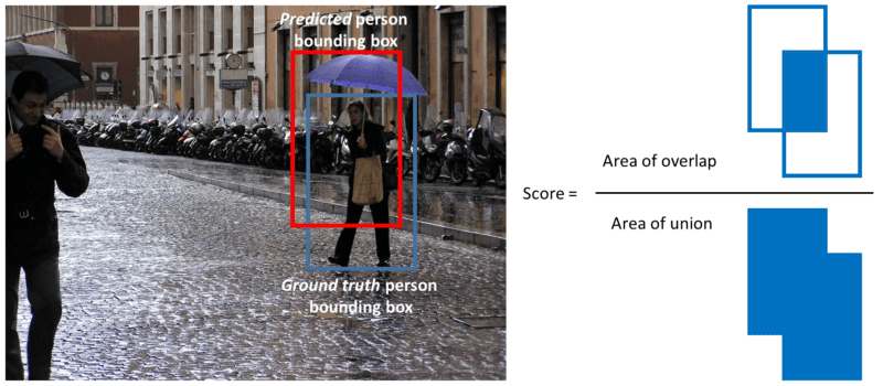
A visualization of the definition of IoU.

Advantages 

• Face Recognition.
• People Counting.
• Industrial Quality Check.
• Self-Driving Cars.
• Security.

Facial Recognition:

A deep learning facial recognition system called the “DeepFace” has been developed by a group of researchers on Facebook, which identifies human faces in a digital image very effectively. Google uses its own facial recognition system in Google Photos, which automatically segregates all the photos based on the person in the image. There are various components involved in Facial Recognition like the eyes, nose, mouth, and eyebrows.

People Counting:

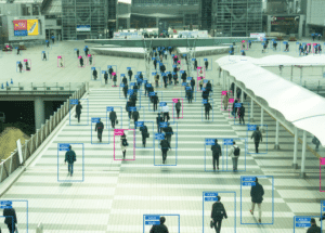
Object detection can be also used for people counting, it is used for analyzing store performance crowd statistics during festivals. These tend to be more difficult as people move out of the frame quickly. It is a very important application, as during crowd gathering this feature can be used for multiple purposes.

Industrial Quality Check:

Object detection is also used in industrial processes to identify products. Finding a specific object through visual inspection is a basic task that is involved in multiple industrial processes like sorting, inventory management, machining, quality management, packaging, etc. Inventory management can be very tricky as items are hard to track in real-time. Automatic object counting and localization allows for improving inventory accuracy.

Self Driving Cars:

Self-driving cars are the future, there’s no doubt in that. But the working behind it is very tricky as it combines a variety of techniques to perceive their surroundings, including radar, laser light, GPS, odometry, and computer vision. Advanced control systems interpret sensory information to identify appropriate navigation paths, as well as obstacles and once the image sensor detects any sign of a living being in its path, it automatically stops. This happens at a very fast rate and is a big step towards Driverless Cars.

Security:

Object Detection plays a very important role in Security. Be it face ID of Apple or the retina scan used in all the sci-fi movies. It is also used by the government to access the security feed and match it with their existing database to find any criminals or to detect the robbers’ vehicle. The applications are limitless.

Conclusion

Now with this, we come to an end to this Object Detection Tutorial. I hope you guys enjoyed this article and understood the power of Tensorflow, and how easy it is to detect objects in images. So, if you have read this, you are no longer a newbie to Object Detection and TensorFlow. Try out these examples and let me know if there are any challenges you are facing while deploying the code.