Artificial Neural Network: A Complete Guide Tutorial For FREE | CHECK-OUT

Last updated on 18th Jul 2020, Blog, Tutorials

Neural networks are parallel computing devices, which are basically an attempt to make a computer model of the brain. The main objective is to develop a system to perform various computational tasks faster than the traditional systems. This tutorial covers the basic concept and terminologies involved in Artificial Neural Network. Sections of this tutorial also explain the architecture as well as the training algorithm of various networks used in ANN.

Neural network

• The neural network is a technology based on the structure of the neurons inside a human brain.
• Neural networks are the most important technique for machine learning and artificial intelligence. They are dramatically improving the state-of-the-art in energy, marketing, health, and many other domains.

Neural network examples

• From simple problems to very complicated ones, neural networks have been used in various industries. Here are several examples of where neural network has been used:
• banking : you can see many big banks betting their future on this technology. From predicting how much money they need to put inside an ATM to optimize their trip back and forth to refill. Into replacing the old technology to detect fraudulent credit card transactions.
• advertising : big advertising companies like Google Adsense deploy neural networks to further optimize their ad choice in relevancy. This results in better targeting and an associated increase in the Click-Through Rate.
• healthcare : many academics and start-ups are trying to solve difficult problems that were unsolved before. Examples include clinical imaging to assist doctors in reading MRIs and genomics where DNA sequences are read.
• automotive : the self-driving car is of huge interest. Huge deal. But I still doubt they can implement those cars in the congestive road of Jakarta…

Structure Of A Neural Network

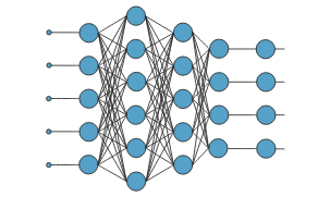
Artificial neural networks are composed of elementary computational units called neurons (McCulloch & Pitts, 1943) combined according to different architectures. For example, they can be arranged in layers (multi-layer network), or they may have a connection topology. Layered networks consist of:

• Input layer, made of n neurons (one for each network input);
• Hidden layer, composed of one or more hidden (or intermediate) layers consisting of m neurons;
• Output layer, consisting of p neurons (one for each network output).

The connection mode allows distinguishing between two types of architectures:

• The feedback architecture, with connections between neurons of the same or previous layer;
• The feed forward architecture (Hornik, Stinchcombe, & White, 1989), without feedback connections (signals go only to the next layer’s neurons).

Types of Neural Networks

There are many types of neural networks available or that might be in the development stage. They can be classified depending on their: Structure, Data flow, Neurons used and their density, Layers and their depth activation filters etc.

       A. Perceptron

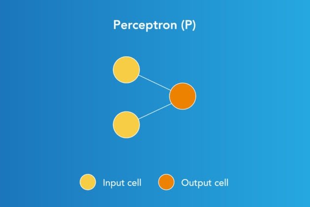
• Perceptron model, proposed by Minsky-Papert is one of the simplest and oldest models of Neuron. It is the smallest unit of neural network that does certain computations to detect features or business intelligence in the input data. It accepts weighted inputs, and apply the activation function to obtain the output as the final result. Perceptron is also known as TLU(threshold logic unit)
• Perceptron is a supervised learning algorithm that classifies the data into two categories, thus it is a binary classifier. A perceptron separates the input space into two categories by a hyperplane represented by the following equation

Advantages of Perception :

Perceptrons can implement Logic Gates like AND, OR, or NAND

Disadvantages of Perception :

Perceptrons can only learn linearly separable problems such as boolean AND problem. For non-linear problems such as boolean XOR problem, it does not work.

B. Feed Forward Neural Networks

• Applications on Feed Forward Neural Networks:
• Simple classification (where traditional Machine-learning based classification algorithms have limitations)
• Face recognition [Simple straight forward image processing]
• Computer vision [Where target classes are difficult to classify]

Speech Recognition :

• The simplest form of neural networks where input data travels in one direction only, passing through artificial neural nodes and exiting through output nodes. Where hidden layers may or may not be present, input and output layers are present there. Based on this, they can be further classified as a single-layered or multi-layered feed-forward neural network.
• Number of layers depends on the complexity of the function. It has uni-directional forward propagation but no backward propagation. Weights are static here. An activation function is fed by inputs which are multiplied by weights. To do so, classifying activation function or step activation function is used. For example:
• The neuron is activated if it is above threshold (usually 0) and the neuron produces 1 as an output. The neuron is not activated if it is below threshold (usually 0) which is considered as -1. They are fairly simple to maintain and are equipped with to deal with data which contains a lot of noise.

Advantages of Feed Forward Neural Networks

• Less complex, easy to design & maintain
• Fast and speedy [One-way propagation]
• Highly responsive to noisy data

Disadvantages of Feed Forward Neural Networks:

Cannot be used for deep learning [due to absence of dense layers and back propagation]

C. Multilayer Perceptron

Applications on Multi-Layer Perceptron

• Speech Recognition
• Machine Translation
• Complex Classification

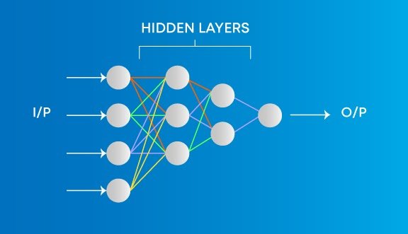
• An entry point towards complex neural nets where input data travels through various layers of artificial neurons. Every single node is connected to all neurons in the next layer which makes it a fully connected neural network. Input and output layers are present having multiple hidden Layers i.e. at least three or more layers in total. It has a bi-directional propagation i.e. forward propagation and backward propagation.
• Inputs are multiplied with weights and fed to the activation function and in backpropagation, they are modified to reduce the loss. In simple words, weights are machine learnt values from Neural Networks. They self-adjust depending on the difference between predicted outputs vs training inputs. Nonlinear activation functions are used followed by softmax as an output layer activation function.

Advantages on Multi-Layer Perceptron:

Used for deep learning [due to the presence of dense fully connected layers and back propagation] 

Disadvantages on Multi-Layer Perceptron: 

Comparatively complex to design and maintain

Comparatively slow (depends on number of hidden layers)

D. Convolutional Neural Network

Applications on Convolution Neural Network

• Image processing
• Computer Vision
• Speech Recognition
• Machine translation
• Convolution neural network contains a three-dimensional arrangement of neurons, instead of the standard two-dimensional array. The first layer is called a convolutional layer. Each neuron in the convolutional layer only processes the information from a small part of the visual field. Input features are taken in batch-wise like a filter. The network understands the images in parts and can compute these operations multiple times to complete the full image processing. Processing involves conversion of the image from RGB or HSI scale to grey-scale. Furthering the changes in the pixel value will help to detect the edges and images can be classified into different categories.

Advantages of Convolution Neural Network:

• Used for deep learning with few parameters
• Less parameters to learn as compared to fully connected layer

Disadvantages of Convolution Neural Network:

• Comparatively complex to design and maintain
• Comparatively slow [depends on the number of hidden layers]

E. Radial Basis Function Neural Networks

Radial Basis Function Network consists of an input vector followed by a layer of RBF neurons and an output layer with one node per category. Classification is performed by measuring the input’s similarity to data points from the training set where each neuron stores a prototype. This will be one of the examples from the training set.

Application: Power Restoration

F. Recurrent Neural Networks

Applications of Recurrent Neural Networks

• Text processing like auto suggest, grammar checks, etc.
• Text to speech processing
• Image tagger
• Sentiment Analysis
• Translation
• Designed to save the output of a layer, Recurrent Neural Network is fed back to the input to help in predicting the outcome of the layer. The first layer is typically a feed forward neural network followed by recurrent neural network layer where some information it had in the previous time-step is remembered by a memory function. Forward propagation is implemented in this case. It stores information required for it’s future use. If the prediction is wrong, the learning rate is employed to make small changes. Hence, making it gradually increase towards making the right prediction during the backpropagation.

Advantages of Recurrent Neural Networks

• Model sequential data where each sample can be assumed to be dependent on historical ones is one of the advantage.  
• Used with convolution layers to extend the pixel effectiveness.

Disadvantages of Recurrent Neural Networks

• Gradient vanishing and exploding problems 
• Training recurrent neural nets could be a difficult task 
• Difficult to process long sequential data using ReLU as an activation function.

Improvement over RNN: LSTM (Long Short-Term Memory) Networks

G. Sequence to sequence models

• A sequence to sequence model consists of two Recurrent Neural Networks. Here, there exists an encoder that processes the input and a decoder that processes the output. The encoder and decoder work simultaneously – either using the same parameter or different ones.
• This model, on contrary to the actual RNN, is particularly applicable in those cases where the length of the input data is equal to the length of the output data. While they possess similar benefits and limitations of the RNN, these models are usually applied mainly in chatbots, machine translations, and question answering systems.

 H. Modular Neural Network 

Applications of Modular Neural Network

• Stock market prediction systems
• Adaptive MNN for character recognitions 
• Compression of high level input data

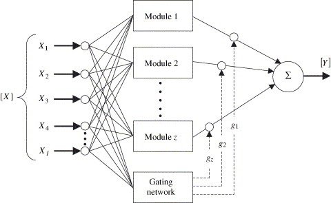
A modular neural network has a number of different networks that function independently and perform sub-tasks. The different networks do not really interact with or signal each other during the computation process. They work independently towards achieving the output.

Advantages of Modular Neural Network

• Efficient
• Independent training
• Robustness

Disadvantages of Modular Neural Network

Moving target Problems

The architecture of an artificial neural network:

To understand the concept of the architecture of an artificial neural network, we have to understand what a neural network consists of. In order to define a neural network that consists of a large number of artificial neurons, which are termed units arranged in a sequence of layers. Lets us look at various types of layers available in an artificial neural network.

Artificial Neural Network primarily consists of three layers:

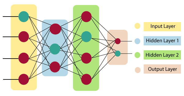
Input Layer:

As the name suggests, it accepts inputs in several different formats provided by the programmer.

Hidden Layer:

The hidden layer presents in-between input and output layers. It performs all the calculations to find hidden features and patterns.

Output Layer:

The input goes through a series of transformations using the hidden layer, which finally results in output that is conveyed using this layer.The artificial neural network takes input and computes the weighted sum of the inputs and includes a bias. This computation is represented in the form of a transfer function.

It determines weighted total is passed as an input to an activation function to produce the output. Activation functions choose whether a node should fire or not. Only those who are fired make it to the output layer. There are distinctive activation functions available that can be applied upon the sort of task we are performing.

Neural network construction

• Now, you know what to do to prepare the data. Let’s get into the action.
• Type jupyter notebook in your command line to get started.

Your browser will open up a window like this. Using Jupyter notebook, you can code Python interactively.

• Then do the set-up imports:

• The fashion MNIST dataset is already included inside Keras’ own collection. For other datasets, you might want to import via OpenCV or Python Image Library to make these ready for processing and training.
• For our fashion MNIST, let’s just load the data:

(x_train, y_train), (x_test, y_test) = fashion_mnist.load_data()

Okay, you are ready now to create your own neural network.

First neural network

• The objective is to build a neural network that will take an image as an input and output whether it is a cat picture or not.
• Feel free to grab the entire notebook and the dataset here. It also contains some useful utilities to import the dataset.

Import the data

As always, we start off by importing the relevant packages to make our code work:

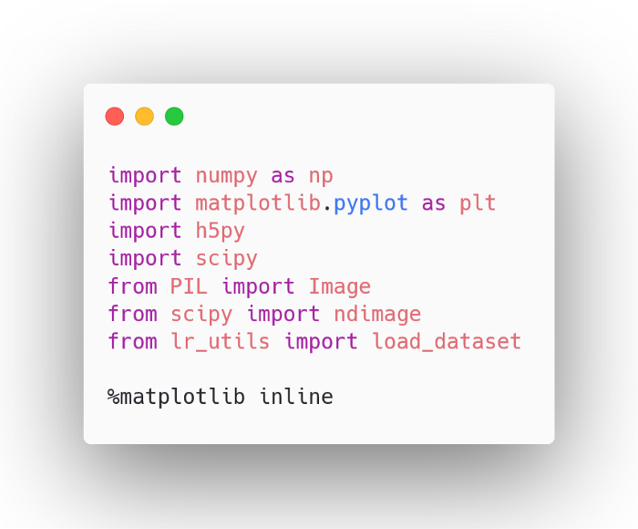
Then, we load the data and see what the pictures look like:

And you should see the following:

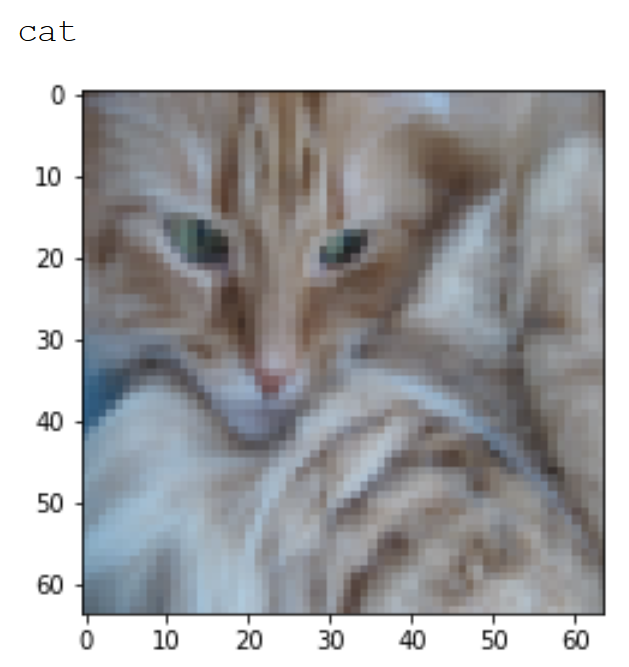
Then, let’s print out more information about the dataset:

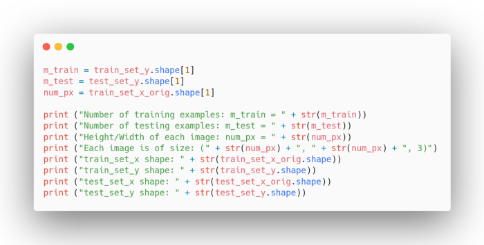
And you should see:

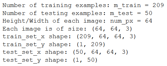
As you can see, we have 209 images in the training set, and we have 50 images for training. Each image is a square of width and height of 64px. Also, you notice that image has a third dimension of 3. This is because the image is composed of three layers: a red layer, a blue layer, and a green layer (RGB).

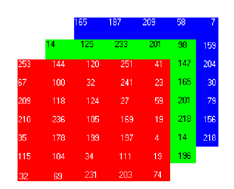
Each value in each layer is between 0 and 255, and it represents how red, or blue, or green that pixel is, generating a unique color for each combination.

Now, we need to flatten the images before feeding them to our neural network:

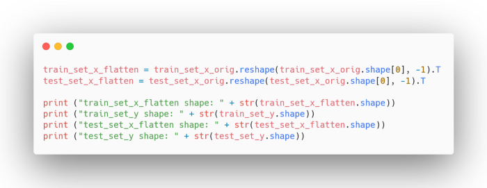
Great! You should now see that the training set has a size of (12288, 209). This means that our images were successfully flatten since

12288 = 64 x 64 x 3.

Finally, we standardize our data set.

Conclusion

So we’ve successfully built a neural network using Python that can distinguish between photos of a cat and a dog. Imagine all the other things you could distinguish and all the different industries you could dive into with that. What an exciting time to live in with these tools we get to play with.