What is Machine Learning? Free Guide Tutorial & REAL-TIME Examples

Last updated on 22nd Jun 2020, Blog, Tutorials

Machine Learning is the field of study that gives computers the capability to learn without being explicitly programmed. ML is one of the most exciting technologies that one would have ever come across. As it is evident from the name, it gives the computer that makes it more similar to humans: The ability to learn. Machine learning is actively being used today, perhaps in many more places than one would expect.

Machine Learning is a system that can learn from example through self-improvement and without being explicitly coded by programmer. The breakthrough comes with the idea that a machine can singularly learn from the data (i.e., example) to produce accurate results.

Machine learning combines data with statistical tools to predict an output. This output is then used by corporate to makes actionable insights. Machine learning is closely related to data mining and Bayesian predictive modeling. The machine receives data as input, use an algorithm to formulate answers.

A typical machine learning tasks are to provide a recommendation. For those who have a Netflix account, all recommendations of movies or series are based on the user’s historical data. Tech companies are using unsupervised learning to improve the user experience with personalizing recommendation.

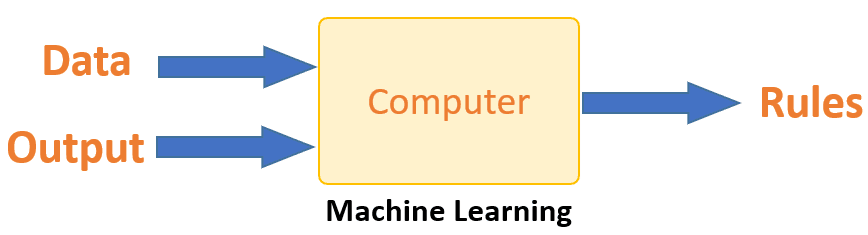
Machine Learning vs. Traditional Programming

Traditional programming differs significantly from machine learning. In traditional programming, a programmer code all the rules in consultation with an expert in the industry for which software is being developed. Each rule is based on a logical foundation; the machine will execute an output following the logical statement. When the system grows complex, more rules need to be written. It can quickly become unsustainable to maintain.

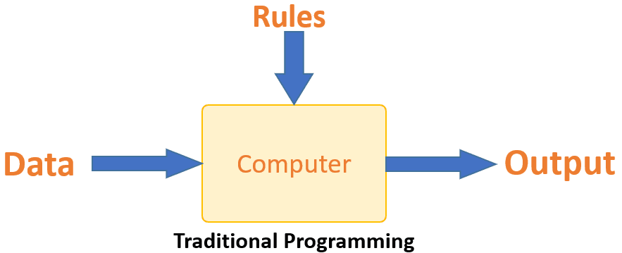
Machine learning is supposed to overcome this issue. The machine learns how the input and output data are correlated and it writes a rule. The programmers do not need to write new rules each time there is new data. The algorithms adapt in response to new data and experiences to improve efficacy over time.

How does Machine learning work?

Machine learning is the brain where all the learning takes place. The way the machine learns is similar to the human being. Humans learn from experience. The more we know, the more easily we can predict. By analogy, when we face an unknown situation, the likelihood of success is lower than the known situation. Machines are trained the same. To make an accurate prediction, the machine sees an example. When we give the machine a similar example, it can figure out the outcome. However, like a human, if its feed a previously unseen example, the machine has difficulties to predict.

The core objective of machine learning is the learning and inference. First of all, the machine learns through the discovery of patterns. This discovery is made thanks to the data. One crucial part of the data scientist is to choose carefully which data to provide to the machine. The list of attributes used to solve a problem is called a feature vector. You can think of a feature vector as a subset of data that is used to tackle a problem.

The machine uses some fancy algorithms to simplify the reality and transform this discovery into a model. Therefore, the learning stage is used to describe the data and summarize it into a model.

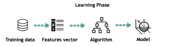
For instance, the machine is trying to understand the relationship between the wage of an individual and the likelihood to go to a fancy restaurant. It turns out the machine finds a positive relationship between wage and going to a high-end restaurant: This is the model

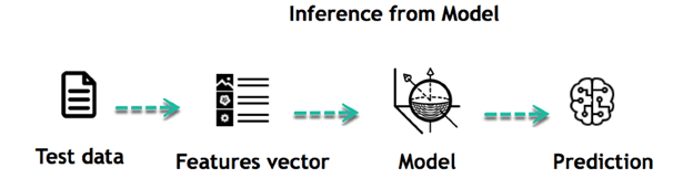
Inferring

When the model is built, it is possible to test how powerful it is on never-seen-before data. The new data are transformed into a features vector, go through the model and give a prediction. This is all the beautiful part of machine learning. There is no need to update the rules or train again the model. You can use the model previously trained to make inference on new data.

The life of Machine Learning programs is straightforward and can be summarized in the following points:

• Define a question
• Collect data
• Visualize data
• Train algorithm
• Test the Algorithm
• Collect feedback
• Refine the algorithm
• Loop 4-7 until the results are satisfying
• Use the model to make a prediction

Once the algorithm gets good at drawing the right conclusions, it applies that knowledge to new sets of data.

Machine learning Algorithms: 

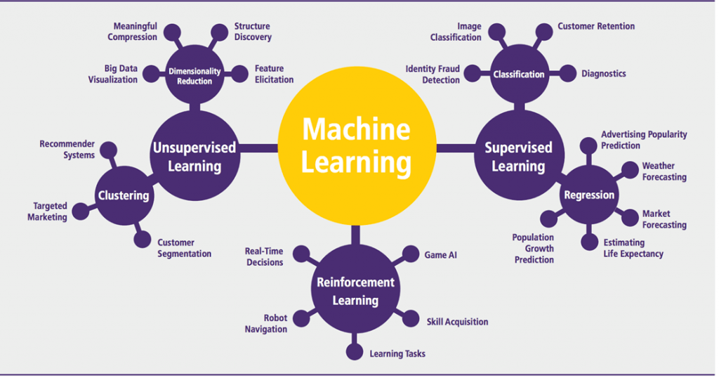
Application of Machine learning:

• Augmentation: Machine learning, which assists humans with their day-to-day tasks, personally or commercially without having complete control of the output. Such machine learning is used in different ways such as Virtual Assistant, Data analysis, software solutions. The primary user is to reduce errors due to human bias.
• Automation: Machine learning, which works entirely autonomously in any field without the need for any human intervention. For example, robots performing the essential process steps in manufacturing plants.
• Finance Industry: Machine learning is growing in popularity in the finance industry. Banks are mainly using ML to find patterns inside the data but also to prevent fraud.
• Government organization: The government makes use of ML to manage public safety and utilities. Take the example of China with the massive face recognition. The government uses Artificial intelligence to prevent jaywalker.
• Healthcare industry: Healthcare was one of the first industry to use machine learning with image detection.
• Marketing: Broad use of AI is done in marketing thanks to abundant access to data. Before the age of mass data, researchers develop advanced mathematical tools like Bayesian analysis to estimate the value of a customer. With the boom of data, marketing department relies on AI to optimize the customer relationship and marketing campaign.

Supervised Machine Learning

In the majority of supervised learning applications, the ultimate goal is to develop a finely tuned predictor function h(x) (sometimes called the “hypothesis”). “Learning” consists of using sophisticated mathematical algorithms to optimize this function so that, given input data x about a certain domain (say, square footage of a house), it will accurately predict some interesting value h(x) (say, market price for said house).

In practice, x almost always represents multiple data points. So, for example, a housing price predictor might take not only square-footage (x1) but also number of bedrooms (x2), number of bathrooms (x3), number of floors (x4), year built (x5), zip code (x6), and so forth. Determining which inputs to use is an important part of ML design. However, for the sake of explanation, it is easiest to assume a single input value is used.

So let’s say our simple predictor has this form:

where θ0 and θ1 are constants. Our goal is to find the perfect values of θ0 and θ1 to make our predictor work as well as possible.

Optimizing the predictor h(x) is done using training examples. For each training example, we have an input value x_train, for which a corresponding output, y, is known in advance. For each example, we find the difference between the known, correct value y, and our predicted value h(x_train). With enough training examples, these differences give us a useful way to measure the “wrongness” of h(x). We can then tweak h(x) by tweaking the values of θ0 and θ1 to make it “less wrong”. This process is repeated over and over until the system has converged on the best values for θ0 and θ1. In this way, the predictor becomes trained, and is ready to do some real-world predicting.

Machine Learning Examples:

We stick to simple problems in this post for the sake of illustration, but the reason ML exists is because, in the real world, the problems are much more complex. On this flat screen we can draw you a picture of, at most, a three-dimensional data set, but ML problems commonly deal with data with millions of dimensions, and very complex predictor functions. ML solves problems that cannot be solved by numerical means alone.

With that in mind, let’s look at a simple example. Say we have the following training data, wherein company employees have rated their satisfaction on a scale of 1 to 100:

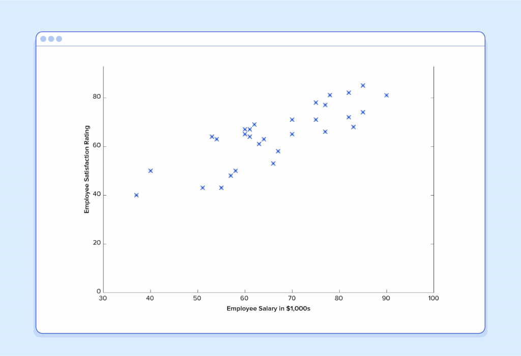
First, notice that the data is a little noisy. That is, while we can see that there is a pattern to it (i.e. employee satisfaction tends to go up as salary goes up), it does not all fit neatly on a straight line. This will always be the case with real-world data (and we absolutely want to train our machine using real-world data!). So then how can we train a machine to perfectly predict an employee’s level of satisfaction? The answer, of course, is that we can’t. The goal of ML is never to make “perfect” guesses, because ML deals in domains where there is no such thing. The goal is to make guesses that are good enough to be useful.

It is somewhat reminiscent of the famous statement by British mathematician and professor of statistics George E. P. Box that “all models are wrong, but some are useful”.

The goal of ML is never to make “perfect” guesses, because ML deals in domains where there is no such thing. The goal is to make guesses that are good enough to be useful.

Machine Learning builds heavily on statistics. For example, when we train our machine to learn, we have to give it a statistically significant random sample as training data. If the training set is not random, we run the risk of the machine learning patterns that aren’t actually there. And if the training set is too small (see law of large numbers), we won’t learn enough and may even reach inaccurate conclusions. For example, attempting to predict company-wide satisfaction patterns based on data from upper management alone would likely be error-prone.

With this understanding, let’s give our machine the data we’ve been given above and have it learn it. First we have to initialize our predictor h(x) with some reasonable values of θ0 and θ1. Now our predictor looks like this when placed over our training set:

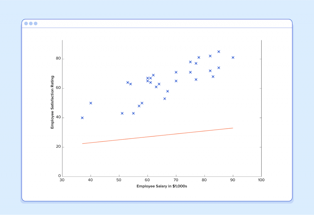
If we ask this predictor for the satisfaction of an employee making $60k, it would predict a rating of 27:

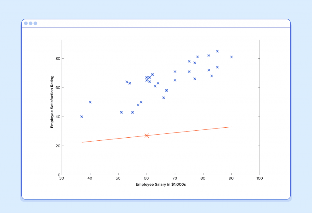
It’s obvious that this was a terrible guess and that this machine doesn’t know very much.

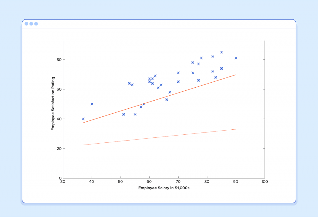
So now, let’s give this predictor all the salaries from our training set, and take the differences between the resulting predicted satisfaction ratings and the actual satisfaction ratings of the corresponding employees. If we perform a little mathematical wizardry (which I will describe shortly), we can calculate, with very high certainty, that values of 13.12 for θ0 and 0.61 for θ1 are going to give us a better predictor.

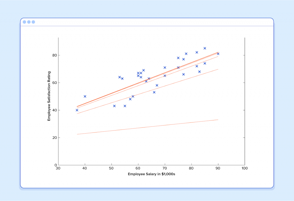
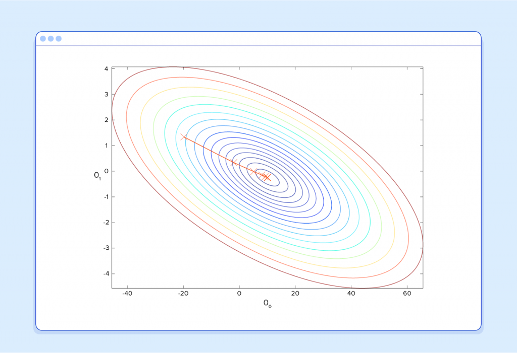
And if we repeat this process, say 1500 times, our predictor will end up looking like this:

At this point, if we repeat the process, we will find that θ0 and θ1 won’t change by any appreciable amount anymore and thus we see that the system has converged. If we haven’t made any mistakes, this means we’ve found the optimal predictor. Accordingly, if we now ask the machine again for the satisfaction rating of the employee who makes $60k, it will predict a rating of roughly 60.

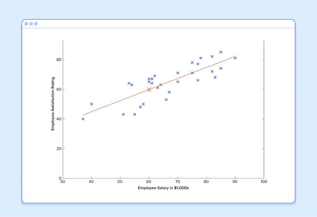
Now we’re getting somewhere.

Machine Learning Regression: A Note on Complexity

The above example is technically a simple problem of univariate linear regression, which in reality can be solved by deriving a simple normal equation and skipping this “tuning” process altogether. However, consider a predictor that looks like this:

This function takes input in four dimensions and has a variety of polynomial terms. Deriving a normal equation for this function is a significant challenge. Many modern machine learning problems take thousands or even millions of dimensions of data to build predictions using hundreds of coefficients. Predicting how an organism’s genome will be expressed, or what the climate will be like in fifty years, are examples of such complex problems.

Many modern ML problems take thousands or even millions of dimensions of data to build predictions using hundreds of coefficients.

Fortunately, the iterative approach taken by ML systems is much more resilient in the face of such complexity. Instead of using brute force, a machine learning system “feels its way” to the answer. For big problems, this works much better. While this doesn’t mean that ML can solve all arbitrarily complex problems (it can’t), it does make for an incredibly flexible and powerful tool.

Gradient Descent – Minimizing “Wrongness”

Let’s take a closer look at how this iterative process works. In the above example, how do we make sure θ0 and θ1 are getting better with each step, and not worse? The answer lies in our “measurement of wrongness” alluded to previously, along with a little calculus.

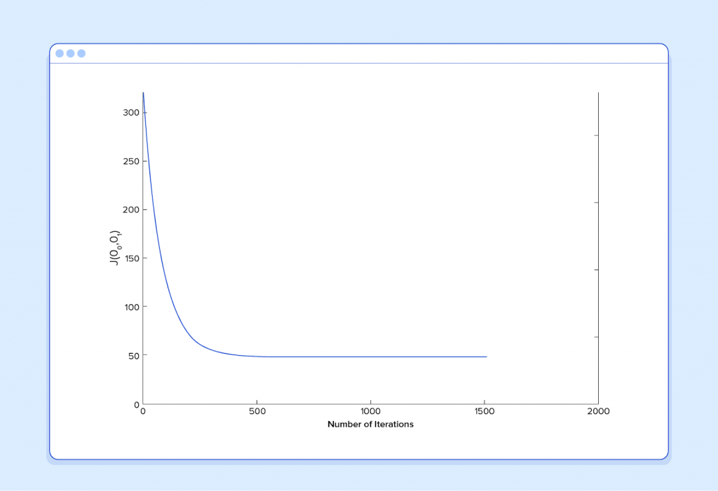
The wrongness measure is known as the cost function (a.k.a., loss function), J(θ). The input θ represents all of the coefficients we are using in our predictor. So in our case,θ is really the pair θ0 and θ1. J( θ0,θ1) gives us a mathematical measurement of how wrong our predictor is when it uses the given values of θ0 and θ1 .

The choice of the cost function is another important piece of an ML program. In different contexts, being “wrong” can mean very different things. In our employee satisfaction example, the well-established standard is the linear least squares function:

With least squares, the penalty for a bad guess goes up quadratically with the difference between the guess and the correct answer, so it acts as a very “strict” measurement of wrongness. The cost function computes an average penalty over all of the training examples.

So now we see that our goal is to find θ0 and θ1 for our predictor h(x) such that our cost function J( θ0,θ1) is as small as possible. We call on the power of calculus to accomplish this.

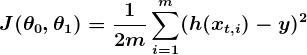
Consider the following plot of a cost function for some particular Machine Learning problem:

Here we can see the cost associated with different values of θ0 and θ1. We can see the graph has a slight bowl to its shape. The bottom of the bowl represents the lowest cost our predictor can give us based on the given training data. The goal is to “roll down the hill”, and find θ0 and θ1 corresponding to this point.

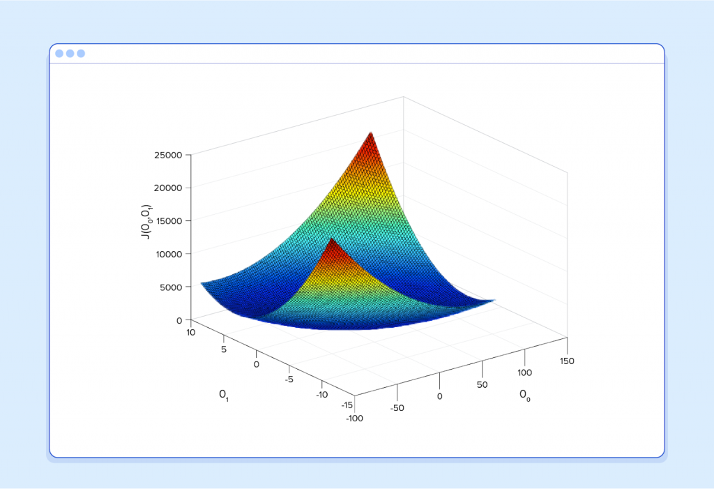
This is where calculus comes in to this machine learning tutorial. For the sake of keeping this explanation manageable, I won’t write out the equations here, but essentially what we do is take the gradient of J(θ0,θ1) , which is the pair of derivatives of J(θ0,θ1)(one over θ0 and one over θ1). The gradient will be different for every different value of θ0 and θ1, and tells us what the “slope of the hill is” and, in particular, “which way is down”, for these particular θs. For example, when we plug our current values of θ into the gradient, it may tell us that adding a little to θ0 and subtracting a little from θ1 will take us in the direction of the cost function-valley floor. Therefore, we add a little to θ0, and subtract a little from θ1, and voilà! We have completed one round of our learning algorithm. Our updated predictor, h(x) = θ0 + θ1x, will return better predictions than before. Our machine is now a little bit smarter.

This process of alternating between calculating the current gradient, and updating the θs from the results, is known as gradient descent.

That covers the basic theory underlying the majority of supervised Machine Learning systems. But the basic concepts can be applied in a variety of different ways, depending on the problem at hand.