Last updated on 24th Jan 2022| 2706
- Introduction to Probability Density Function
- What is Probability Density function
- Process Capability
- Process Performancel
- Concerning The Probability Density Function In Statistics
- Factors of Probability Density Function
- History
- How to Find the Probability Density Function in Statistics?
- What Is the Probability Density Function?
- Articulation for Probability Density Functions
- Properties of a Probability Density Function
- How to Find the Probability Density Function in Statistics?
- What is the utilization of Probability density work?
- Advantage of Probability Density Function
- Prerequisites of Probability Density Function
- Conclusion
- Histogram plots give a quick and solid method for imagining the Probability density of an informal test.
- Parametric Probability density assessment includes choosing a typical circulation and assessing the boundaries for the density work from an information test.
- Nonparametric Probability density assessment includes utilizing a strategy to fit a model to the self-assertive circulation of the information, similar to portion density assessment.
- A persistent arbitrary variable takes on an uncountably limitless number of potential qualities. For a discrete arbitrary variable X that takes on a limited or countably endless number of potential qualities, we decided P(X=x) for each of the potential upsides of X and called it the Probability density mass capacity (“p.m.f.”).
- For consistent irregular factors, as we will before long see, the Probability density that X takes on a specific worth x is 0. That is, tracking down P(X=x) for a ceaseless irregular variable X won’t work. All things considered, we’ll have to track down the Probability density that X falls in some stretch (a,b), that is, we’ll have to track down P(a<'X<'b). We'll do that utilizing a Probability density work ("p.d.f."). We'll initially spur a p.d.f. with a model, and afterward, we'll officially characterize it.
- Cp=min[USL−μ3×σ,μ−LSL3×σ]Cp=min[USL−μ3×σ,μ−LSL3×σ]
- USLUSL = Upper Specification Limit.
- LSLLSL = Lower Specification Limit.
- μμ = assessed mean of the interaction.
- σσ = assessed changeability of the cycle, standard deviation.
- Pp=USL−LSL6×σPp=USL−LSL6×σ
- USLUSL = Upper Specification Limit.
- LSLLSL = Lower Specification Limit.
- σσ = assessed fluctuation of the interaction, standard deviation.
- The higher the worth of cycle execution file PpPp, the better is the interaction.
- P(a) <= X <= P(b)
- In Probability density hypothesis, a Probability density work (PDF), or density of a constant arbitrary variable, is a capacity whose esteem at some random example (or point) in the example space (the arrangement of potential qualities taken by the irregular variable) can be deciphered as giving a relative probability that the worth of the irregular variable would be near that sample.[2][3] at the end of the day, while the outright probability for a consistent irregular variable to take on a specific worth is 0 (since there is a boundless arrangement of potential qualities in any case), the worth of the PDF at two unique examples can be utilized to surmise, in a specific draw of the irregular variable, the amount almost certain it is that the arbitrary variable would be near one example contrasted with the other example.
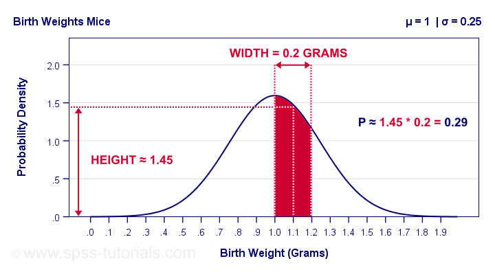
- In a more exact sense, the PDF is utilized to determine the Probability density of the arbitrary variable falling inside a specific scope of qualities, instead of taking on anyone worth. This Probability density is given by the indispensable of this current variable’s PDF over that range-that is, it is given by the region under the density work yet over the flat pivot and between the least and most prominent upsides of the reach. The Probability density work is nonnegative all over the place, and its fundamental over the whole space is equivalent to one.
- The expressions “Probability density dispersion function” and “Probability density function” have likewise here and there been utilized to signify the Probability density work. Notwithstanding, this utilization isn’t standard among probability and analysts. In different sources, “Probability density circulation work” might be utilized when the Probability density conveyance is characterized as a capacity over broad arrangements of qualities or it might allude to the total dispersion capacity, or it could be a Probability density mass capacity (PMF) rather than the density. “Density work” itself is likewise utilized for the Probability density mass capacity, prompting further confusion. overall, however, the PMF is utilized with regards to discrete irregular factors (arbitrary factors that take esteems on a countable set), while the PDF is utilized with regards to constant irregular factors.
- one. Smoothing Parameter (data transmission): Controls the number of tests used to appraise the Probability density of another point.
- 2. Basis Function: Helps to control the circulation of tests.
- Discrete Variable
- Continuous Variable
- P(a) <= X <= P(b)
- The f(x) incentive for every conceivable worth of the arbitrary variable should be positive (non-negative).
- The necessary worth of the complete region of the bend (basic of all potential upsides of the irregular variable) should be one.
- Instructor-led Sessions
- Real-life Case Studies
- Assignments
- The worth of the irregular variable lies among an and b.
- Assuming X signifies the Probability density of choosing a specific number from the reach (stretch) r and s, then, at that point, the Probability density capacity can be communicated as
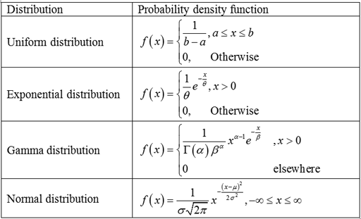
- f(x) = one/(sr) for r < x < s and f(x) = 0 for x < r or x > s.
- The PDF F is addressed as:
- F(x) = P{X ≤ x}
- which is known as the dissemination work or the total conveyance capacity of X.
- The assumption for the arbitrary variable is indicated as,
- In this manner, all discrete and arbitrary factors can be dealt with consistently with the assistance of a consolidated hypothesis.
- It’s an ideal opportunity to perform non-parametric assessments now. You start by bringing in certain modules required for it.
- To perform non-parametric assessments, you should utilize two typical examples and combine them to get an example that doesn’t fit any known normal dispersion.
- Presently, use Kernel density assessment to get a model, which you can then fit your example to make a Probability density appropriation bend.
- You will currently observe the Probability density conveyance for our piece density assessment work.
- You can see that the assessment of part density assessment fits the examples pretty well. To additional tweak the fit, you can change the data transmission of the capacity.
- The Probability density work is utilized in the yearly demonstrating of environmental NO fixation levels.
- Demonstrating diesel motor ignition.
- In measurements, the Probability density work is utilized to decide the conceivable outcomes of the result of an arbitrary variable.
- Probability density Functions are a factual measure used to check the logical result of a discrete worth (e.g., the cost of a stock or ETF). PDFs are plotted on a diagram regularly looking like a ringer bend, with the Probability density of the results lying beneath the bend.
- All the more definitively, since the outright probability of a persistent irregular variable taking on a particular worth is zero because of the limitless arrangement of potential qualities accessible, the worth of a PDF can be utilized to decide the probability of an arbitrary variable falling inside a particular scope of qualities.
- This approach is theoretically basic and helpful for straightforward certifiable models. For individuals without a foundation in arithmetic or measurements, this is, by a wide margin, the most straightforward to process and apply to fundamental certifiable models.
- This approach addresses a portion of the issues of the Classical methodology. The Frequentist approach can deal with circumstances in which results are not similarly logical since it is just worried about the event of an occasion. This approach is additionally ready to deal with probabilities that don’t manage a solitary result. For instance, on the off chance that the occasion is “An arbitrarily picked positive whole number is even”, even though there is no specific result of interest – since there are endlessly numerous numbers – the occasion’s Probability density can in any still up in the air by testing progressively bigger quantities of numbers. As we test an ever-increasing number of numbers, the Probability density will move toward 1/2.
- The idea of rehashing a trial an endless number of times is a psychological study, not something that should be possible. We can lead an enormous number of preliminaries, obviously, never a boundless number of them.
- Thus, when we attempt to assess probabilities, the got amount won’t meet, and will rather sway around the “valid” Probability density of the occasion. It is hard to evaluate this level of vulnerability without circularly utilizing Probability density.
- In this instructional exercise on ‘All that You Need to Know About the Probability Density Function’, you comprehended a Probability density work in insights. You then, at that point, took a gander at how to observe the Probability density work in measurements and python.
- Assuming you are enthused about finding out with regards to Probability density work and related factual ideas, you could investigate a vocation. Sampliner’s Post Graduate Program in Data Analytics is one of the most complete web-based projects out there for this. To dive deeper into insights and ordinary circulation, share your questions with us by referencing them in this current page’s remarks area.
- We will have our specialists survey them at the earliest. You can likewise comprehend the idea of the Probability density work and other measurable ideas by looking at this video on our YouTube channel.
Introduction to Probability Density Function:
In this instructional exercise, you will find a delicate prologue to Probability density assessment. In the wake of finishing this instructional exercise, you will know:
What is Probability Density function:
Process Capability:
Process capacity can be characterized as a quantifiable property of a cycle comparative with its particular. It is communicated as an interaction capacity file CpCp. The interaction capacity file is utilized to check the fluctuation of the result created by the cycle and to contrast the variability and the item resistance. CpCp is administered by the following equation:
Higher the worth of interaction ability to record CpCp, the better is the cycle.
Example:
Consider the instance of a vehicle and its parking structure. carport size expresses as far as possible and vehicle characterizes the cycle yield. Here process capacity will tell the relationship between vehicle size, carport size, and how a long way from the center of the carport you can leave the vehicle. If vehicle size is litter more modest than carport size, you can undoubtedly squeeze your vehicle into it. On the off chance that vehicle size is tiny contrasted with carport size, it can fit from any separation from focus. In terms of the cycle of control, such interaction with little variety permits to leave vehicle effectively in a carport and meets the client’s prerequisite. How about we see the above-expressed model as far as cycle ability file CpCp.
Cp=12Cp=12 – carport size is more modest than vehicle and can not accommodate your vehicle.
Cp=1Cp=1 – carport size is only adequate for a vehicle and can accommodate your vehicle as it were.
Cp=2Cp=2 – carport size is twice that of your vehicle and can accommodate two vehicles all at once.
Cp=3Cp=3 – carport size is multiple times than your vehicle and can accommodate three vehicles all at once.
Process Performance:
Process execution attempts to check the conformance of the example created utilizing the interaction. It is communicated as an interaction execution record PpPp. It checks whether or not it is meeting client necessities. It differs from Process Capability in the way that Process Performance is relevant to a specific group of material. A testing strategy might be very substantial to help the variety in the group. Process Performance is just to be utilized when a cycle control can’t be assessed. PpPp is administered by the following equation:
Concerning The Probability Density Function In Statistics:
F or discrete factors, the Probability density is direct and can be determined without any problem. Be that as it may, for ceaseless factors which can take on boundless qualities, the Probability density additionally takes on a scope of endless qualities. The capacity which depicts the Probability density for such factors is known as a Probability density work in measurements.
Factors of Probability Density Function:
A capacity that characterizes the connection between an arbitrary variable and its Probability density , to such an extent that you can track down the Probability density of the variable utilizing the capacity, is known as a Probability Density Function (PDF) in insights. The various kinds of factors. They are for the most of two sorts:

Learn Advanced Python and Statistics for Financial Analysis Certification Training Course to Build Your Skills
Weekday / Weekend BatchesSee Batch DetailsDiscrete Variable:
A variable that can take on a specifically limited worth inside a particular reach is known as a discrete variable. It normally isolates the qualities by a limited span, e.g., an amount of two dice. On moving two dice and including the subsequent result, the outcome can have a place with a bunch of numbers not surpassing one2 (as the greatest aftereffect of a dice toss is 6). The qualities are additionally positive.
Continuous Variable:
A consistent irregular variable can take on limitless various qualities inside the scope of qualities, e.g., the measure of precipitation happening in a month. The downpour noticed can be one.7cm, yet the specific worth isn’t known. It can be one.70one, one.7687, and so on All things considered, you can characterize the scope of qualities it falls into. Inside this worth, it can take on limitless various qualities.
History:
How to Find the Probability Density Function in Statistics?
The following are three primary advances:
Summing up the density with a histogram: Your initial believer the information into the discrete structure by plotting it as a histogram. A histogram is a chart with downright qualities on the x-pivot and receptacles of various statures, providing you with an include of the qualities in that classification. The quantity of canisters is critical as it decides the number of bars the histogram will have and their width. This will let you know how it will plot your density.
Performing Parametric density assessment: A PDF can take on a shape like numerous standard capacities. The state of the histogram will assist you with figuring out which sort of capacity it is. You can compute the boundaries related to the capacity to get our density.
To check to assume our histogram is an astounding fit for the capacity, you can:
1. Plot the density capacity and look at histogram shape
2. Compare examples of the capacity with real examples
3. Use a measurable test
Performing Non-Parametric Density Estimation: In situations where the state of the histogram doesn’t match a typical Probability density work, or can’t be made to fit one, you compute the density involving every one of the examples in the information and apply specific calculations. One such calculation is the Kernel Density Estimation. It utilizes a numerical capacity to compute and smooth probabilities so their total is one all the time. To do this, you want the accompanying boundaries:
All that You Need to Know About the Probability Density Function in Statistics. For discrete factors, the Probability density is direct and can be determined without any problem. In any case, for consistent factors which can take on limitless qualities, the Probability density additionally takes on a scope of endless qualities. The capacity which depicts the Probability density for such factors is known as a Probability density work in measurements.
What Is the Probability Density Function?
A capacity that characterizes the connection between an arbitrary variable and its Probability density, to such an extent that you can track down the Probability density of the variable utilizing the capacity, is known as a Probability Density Function (PDF) in insights. The various sorts of factors. They are basically of two sorts:
1. Discrete Variable: A variable that can take on a specifically limited worth inside a particular reach is known as a discrete variable. It typically isolates the qualities by a limited stretch, e.g., an amount of two dice. On moving two dice and including the subsequent result, the outcome can have a place with a bunch of numbers not surpassing one2 (as the greatest aftereffect of a dice toss is 6). The qualities are additionally unequivocal.
2. Continuous Variable: A constant arbitrary variable can take on endless various qualities inside the scope of qualities, e.g., a measure of precipitation happening in a month. The downpour noticed can be one.7cm, yet the specific worth isn’t known. It can be one.70one, one.7687, and so forth Accordingly, you can characterize the scope of qualities it falls into. Inside this worth, it can take on endless various qualities.
Conditions to be Satisfied by a capacity to be viewed as a Probability Density Function:
The worth of a discrete variable can be precisely estimated as opposed to a ceaseless variable that can have a boundless number of qualities. Any capacity ought to fulfill the under two conditions to be a Probability density work:
Articulation for Probability Density Functions:
Assuming the irregular variable is discrete, its Probability density appropriation is called Probability density mass capacity, and if it is a constant variable, the Probability density conveyance is called Probability density work. A PDF is involved when the arbitrary variable being referred to has a scope of potential qualities. Their Probability density appropriation is utilized to decide the specific worth. Leave the arbitrary variable alone signified by X. The Probability density work, f of the irregular variable X can be communicated as.

Get JOB Oriented Python and Statistics for Financial Analysis Training for Beginners By MNC Experts
Considering the irregular variable X has a Probability density dissemination work f(x), then, at that point, the connection among f and F can be set up as F′(.x) = f(x). The conveyance capacity of a discrete irregular variable is not the same as its Probability density dispersion work. The connection between the two can be communicated as beneath:
The equation of Probability Density Function:
The Probability density of a persistent irregular variable X on some proper worth x is 0 all of the time. For this situation, P(X = x) can’t be utilized. The worth of the X lying between a scope of qualities (a,b) ought not entirely settled. To decide something similar, the accompanying equation is utilized.
Properties of a Probability Density Function:
A persistent arbitrary variable that takes its worth between the reach (a,b), for example, will be assessed by computing the region under the bend and the X-pivot plotted with (a) as its lower breaking point and (b) as its furthest cutoff. The Probability density work for the above is addressed as:
The Probability density work is positive (non-negative) for every conceivable worth. This implies f(x)≥ 0, for each x. The region falling between the density bend and the X-hub (even hub) approaches one.
How to Find the Probability Density Function in Statistics?
The following are three primary advances:
Summing up the density with a histogram:
You initially proselyte the information into the discrete structure by plotting it as a histogram. A histogram is a chart with clear cut qualities on the x-pivot and containers of various statures, providing you with an include of the qualities in that classification. The quantity of canisters is critical as it decides the number of bars the histogram will have and their width. This will let you know how it will plot your density.
Performing Parametric density assessment:
A PDF can take on a shape like numerous standard capacities. The state of the histogram will assist you with figuring out which sort of capacity it is. You can compute the boundaries related to the capacity to get our density. To check to assume our histogram is a magnificent fit for the capacity, you can:
1. Plot the density capacity and think about histogram shape
2. Compare examples of the capacity with real examples
3. Use a measurable test
Performing Non-Parametric Density Estimation:
In situations where the state of the histogram doesn’t match a typical Probability density work, or can’t be made to fit one, you compute the density involving every one of the examples in the information and apply specific calculations. One such calculation is the Kernel Density Estimation. It utilizes a numerical capacity to compute and smooth probabilities so their aggregate is one one00% of the time.
To do this, you want the accompanying boundaries:
Smoothing Parameter (data transfer capacity): Controls the number of tests used to assess the Probability density of another point.
Basis Function: Helps to control the appropriation of tests.You would need to expect the example to be of another appropriation and rehash the interaction.
Performing Non-Parametric Density Estimation:
Creating a Kernel Density Estimation Function:
Uses of Probability Density Function:
What is the utilization of Probability density work?
Advantage of Probability Density Function:
The straightforwardness of this understanding cutoff points it in more than one way. It can’t deal with occasions with a limitless number of potential results. It additionally can’t deal with occasions where every result isn’t similarly possible, for example, tossing a weighted bite the dust. These impediments make it irrelevant for more convoluted errands. Although this approach develops the Classical methodology, it has a few restrictions.
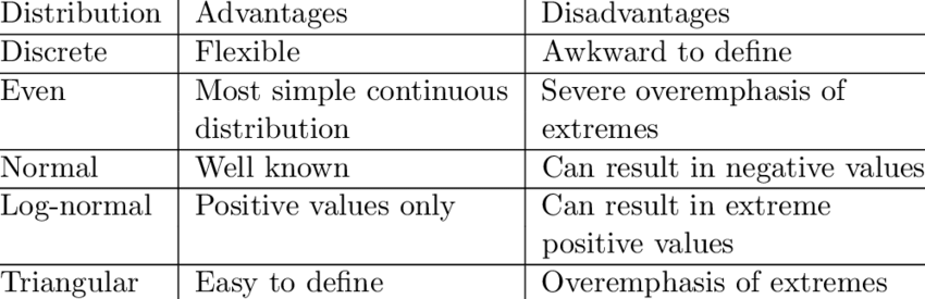
Disadvantage of Probability Density Function:
Prerequisites of Probability Density Function:
Before continuing with this instructional exercise, you ought to have an essential comprehension of Mathematics.