Last updated on 03rd Jan 2022| 1897
Machine learning is important because it gives enterprises a view of trends in customer behavior and business operational patterns, as well as supports the development of new products. Many of today’s leading companies, such as Facebook, Google and Uber, make machine learning a central part of their operations. Machine learning has become a significant competitive differentiator for many companies.
- Introduction
- Top Ten Techniques of Machine Learning
- Conclusion
Introduction :-
AI Techniques (like Regression, Classification, Clustering, Anomaly recognition, and so on) are utilized to assemble the preparation information or a numerical model utilizing specific calculations dependent on the calculations measurement to make forecast without the need of programming, as these strategies are compelling in making the framework modern, models and advances robotization of things with decreased expense and labor.
- Linear Regression
- Logistic Regression
- Linear Discriminant Analysis
- Classification and Regression Trees
- Naive Bayes
- K-Nearest Neighbors (KNN)
- Learning Vector Quantization (LVQ)
- Support Vector Machines (SVM)
- Random Forest
- Boosting
- AdaBoost
Top Ten Techniques of Machine Learning:-
- Linear relapse is maybe one of the most notable and surely known calculations in insights and AI.
- Prescient demonstrating is fundamentally worried about limiting the blunder of a model or making the most dependable expectations conceivable, to the detriment of reasonableness. We will acquire, reuse and take calculations from a wide range of fields, including measurements and use them towards these closures.
- The portrayal of direct relapse is a condition that depicts a line that best fits the connection between the information factors (x) and the result factors (y), by observing explicit weightings for the information factors called coefficients (B).
- We will anticipate y given the information x and the objective of the Linear relapse learning calculation is to track down the qualities for the coefficients B0 and B1
- Various strategies can be utilized to take in the direct relapse model from information, like a Linear polynomial math answer for normal least squares and angle drop advancement.
- Linear relapse has been around for over 200 years and has been broadly considered. Some great basic guidelines when utilizing this method are to eliminate factors that are practically the same (associated) and to eliminate commotion from your information, if conceivable. It is a quick and Linearforward procedure and great first calculation to attempt.
1. Linear Regression:
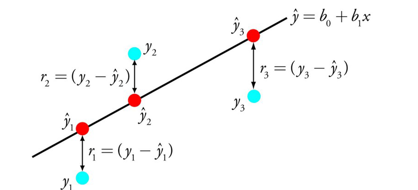
- For instance: y = B0 + B1 * x
- Calculated relapse is one more strategy acquired by AI from the field of measurements. It is the go-to strategy for parallel grouping (issues with two class esteems).
- Calculated relapse resembles direct relapse in that the objective is to observe the qualities for the coefficients that weight each info variable. Dissimilar to direct relapse, the forecast for the result is changed utilizing a non-Linear capacity called the calculated capacity.
- The Logistic capacity appears as though a major S and will change any worth into the reach 0 to 1. This is helpful on the grounds that we can apply a standard to the result of the Logistic capacity to snap esteems to 0 and 1 (for example In the event that under 0.5, yield 1) and foresee a class esteem.
- Due to how the model is taken in, the expectations made by Logistic relapse can likewise be utilized as the likelihood of a given information example having a place with class 0 or class 1. This can be valuable for issues where you want to give more reasoning for a forecast.
- Like direct relapse, calculated relapse takes care of business better when you eliminate credits that are irrelevant to the result variable just as characteristics that are practically the same (connected) to one another. It’s a quick model to learn and successful on double grouping issues.
2. Logistic Regression:
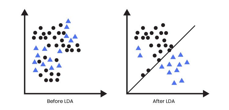
- Calculated Regression is an order calculation generally restricted to just two-class characterization issues. Assuming that you have multiple classes then the Linear Discriminant Analysis calculation is the favored Linear grouping procedure.
- The portrayal of LDA is Linear forward. It comprises of factual properties of your information, determined for each class. For a solitary info variable this incorporates:
- The mean incentive for each class.
- The difference determined across all classes.
- Expectations are made by ascertaining a segregate an incentive for each class and making a forecast for the class with the biggest worth. The procedure expects that the information has a Gaussian dissemination (ringer bend), so it is really smart to eliminate anomalies from your information before hand. It’s a Linearforward and strong technique for grouping prescient demonstrating issues.
3. Linear Discriminant Analysis:
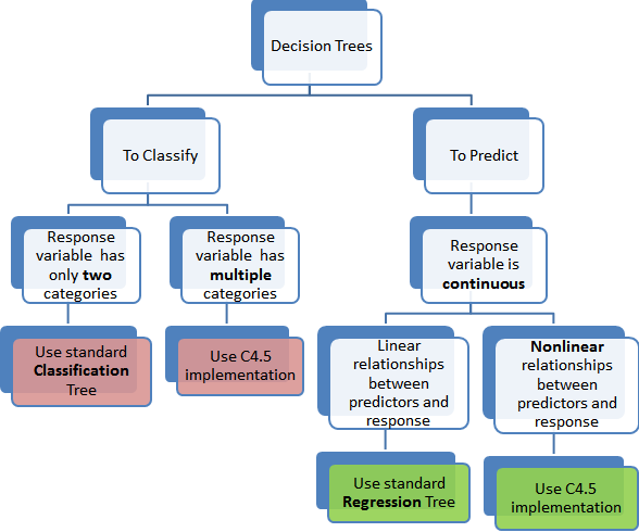
- Choice Trees are a significant kind of calculation for prescient demonstrating AI.
- The portrayal of the choice tree model is a paired tree. This is your paired tree from calculations and information structures, nothing excessively extravagant. Every hub addresses a solitary information variable (x) and a split point on that factor (expecting the variable is numeric).
- The leaf hubs of the tree contain a result variable (y) which is utilized to make an expectation. Expectations are made by strolling the parts of the tree until showing up at a leaf hub and result the class esteem at that leaf hub.
- Trees are quick to learn and exceptionally quick for making forecasts. They are additionally regularly precise for an expansive scope of issues and don’t need any exceptional groundwork for your information.
4. Classification and Regression Trees:

Develop Your Skills with Advanced Machine Learning Certification Training
Weekday / Weekend BatchesSee Batch Details- Innocent Bayes is a basic yet shockingly strong calculation for prescient displaying.
- The model is contained two kinds of probabilities that can be determined Linearforwardly from your preparation information: 1) The likelihood of each class; and 2) The contingent likelihood for each class given every x worth. When determined, the likelihood model can be utilized to make expectations for new information utilizing Bayes Theorem. At the point when your information is genuine esteemed it is normal to accept a Gaussian dispersion (chime bend) so you can undoubtedly appraise these probabilities.
- Gullible Bayes is called innocent since it accepts that each info variable is autonomous. This is a solid presumption and unreasonable for genuine information, by the by, the strategy is exceptionally compelling on a huge scope of intricate issues.
5. Naive Bayes:
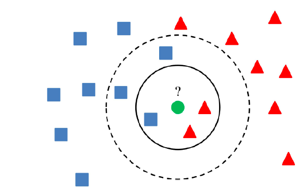
- Expectations are made for another important informative element via looking through the whole preparing set for the K most comparable occasions (the neighbors) and summing up the result variable for those K examples. For relapse issues, this may be the mean result variable, for characterization issues this may be the mode (or generally normal) class esteem.
- The stunt is in how to decide the closeness between the information occasions. The least difficult strategy assuming that your traits are the entirety of a similar scale (all in creeps for instance) is to utilize the Euclidean distance, a number you can ascertain Linearforwardly dependent on the contrasts between each information variable.
- KNN can require a great deal of memory or space to store the entirety of the information, however just plays out an estimation (or realize) when an expectation is required, in the nick of time. You can likewise refresh and arrange your preparation occurrences after some time to keep expectations precise.
- Distance or closeness can separate in extremely high aspects (heaps of information factors) which can contrarily influence the presentation of the calculation on your concern. This is known as the scourge of dimensionality. It recommends you just utilize those information factors that are generally pertinent to foreseeing the result variable.
6. K-Nearest Neighbors:
- A disadvantage of K-Nearest Neighbors is that you really want to hold tight to your whole preparing dataset. The Learning Vector Quantization calculation (or LVQ for short) is a fake neural organization calculation that permits you to pick the number of preparing examples to cling to and realizes precisely what those occasions ought to resemble.
- The portrayal for LVQ is an assortment of codebook vectors. These are chosen haphazardly to start with and adjusted to best sum up the preparation dataset over various cycles of the learning calculation. Later educated, the codebook vectors can be utilized to make forecasts very much like K-Nearest Neighbors. The most comparable neighbor (best matching codebook vector) is found by working out the distance between each codebook vector and the new information occasion. The class worth or (genuine worth on account of relapse) for the best matching unit is then returned as the forecast. Best outcomes are accomplished in the event that you rescale your information to have a similar reach, for example, somewhere in the range of 0 and 1.
- Assuming you find that KNN gives great outcomes on your dataset take a stab at utilizing LVQ to lessen the memory prerequisites of putting away the whole preparing dataset.
7. Learning Vector Quantization:
- Support Vector Machines are maybe one of the most famous and discussed AI calculations.
- A hyperplane is a line that parts the information variable space. In SVM, a hyperplane is chosen to best separate the focuses in the information variable space by their group, either class 0 or class 1. In two-aspects, you can envision this as a line and how about we expect that every one of our feedback focuses can be totally isolated by this line. The SVM learning calculation tracks down the coefficients that outcomes in the best division of the classes by the hyperplane.
- The distance between the hyperplane and the nearest information focuses is alluded to as the edge. The best or ideal hyperplane that can isolate the two classes is the line that has the biggest edge. Just these focuses are important in characterizing the hyperplane and in the development of the classifier. These focuses are known as the help vectors. They support or characterize the hyperplane. By and by, an advancement calculation is utilized to observe the qualities for the coefficients that boosts the edge.
- SVM may be one of the most remarkable out-of-the-crate classifiers and worth taking a stab at your dataset.
8. Support Vector Machines:
- Random Forest is one of the most well known and most remarkable AI calculations. It is a kind of outfit AI calculation called Bootstrap Aggregation or sacking.
- The bootstrap is a strong measurable technique for assessing an amount from an information test. Like a mean. You take bunches of tests of your information, compute the mean, then, at that point, normal each of your mean qualities to provide you with a superior assessment of the genuine mean worth.
- In packing, a similar methodology is utilized, however rather for assessing whole measurable models, most generally choice trees. Various examples of your preparation information are taken then models are built for every information test. At the point when you really want to make a forecast for new information, each model makes an expectation and the forecasts are found the middle value of to give a superior gauge of the genuine result esteem.
- Random timberland is a change on this methodology where choice trees are made so that rather than choosing ideal split focuses, problematic parts are made by presenting haphazardness.
- The models made for each example of the information are in this manner more not quite the same as they in any case would be, yet at the same time precise in their remarkable and various ways. Consolidating their expectations brings about a superior gauge of the genuine fundamental result esteem.
- Assuming you get great outcomes with a calculation with high change (like choice trees), you can frequently improve results by stowing that calculation.
9. Bagging and Random Forest:
- A disadvantage of K-Nearest Neighbors is that you really want to hold tight to your whole preparing dataset. The Learning Vector Quantization calculation (or LVQ for short) is a fake neural organization calculation that permits you to pick the number of preparing examples to cling to and realizes precisely what those occasions ought to resemble.
- The portrayal for LVQ is an assortment of codebook vectors. These are chosen haphazardly to start with and adjusted to best sum up the preparation dataset over various cycles of the learning calculation. Later educated, the codebook vectors can be utilized to make forecasts very much like K-Nearest Neighbors. The most comparable neighbor (best matching codebook vector) is found by working out the distance between each codebook vector and the new information occasion. The class worth or (genuine worth on account of relapse) for the best matching unit is then returned as the forecast. Best outcomes are accomplished in the event that you rescale your information to have a similar reach, for example, somewhere in the range of 0 and 1.
- Assuming you find that KNN gives great outcomes on your dataset take a stab at utilizing LVQ to lessen the memory prerequisites of putting away the whole preparing dataset.
10. Boosting and AdaBoost:
Helping is a gr
Conclusion :-
AdaBoost was the first truly effective helping calculation created for parallel grouping. It is the best beginning stage for comprehension helping. Current helping strategies expand on AdaBoost, most quite stochastic slope supporting machines.
oup procedure that endeavors to make a solid classifier from various powerless classifiers. This is finished by building a model from the preparation information, then, at that point, making a second model that endeavors to address the mistakes from the main model. Models are added until the preparation set is anticipated flawlessly or a most extreme number of models are added.
AdaBoost was the first truly effective helping calculation created for parallel grouping. It is the best beginning stage for comprehension helping. Current helping strategies expand on AdaBoost, most quite stochastic slope supporting machines.