Machine Learning Random Forest: A Concise Tutorial Just An Hour

Last updated on 22nd Jun 2020, Blog, Tutorials

What is the Random Forest Algorithm?

Random forests or random decision forests are an ensemble learning method for classification, regression and other tasks that operate by constructing a multitude of decision trees at training time and outputting the class that is the mode of the classes or mean prediction of the individual trees. 

Introduction:

Random forest is a supervised learning algorithm which is used for both classification as well as regression. But however, it is mainly used for classification problems. As we know that a forest is made up of trees and more trees means more robust forest. Similarly, a random forest algorithm creates decision trees on data samples and then gets the prediction from each of them and finally selects the best solution by means of voting. It is an ensemble method which is better than a single decision tree because it reduces the over-fitting by averaging the result.

Working of Random Forest Algorithm:

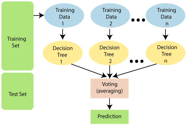
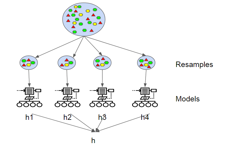
We can understand the working of Random Forest algorithm with the help of following steps −

• Step 1 − First, start with the selection of random samples from a given dataset.
• Step 2 − Next, this algorithm will construct a decision tree for every sample. Then it will get the prediction result from every decision tree.
• Step 3 − In this step, voting will be performed for every predicted result.
• Step 4 − At last, select the most voted prediction result as the final prediction result.

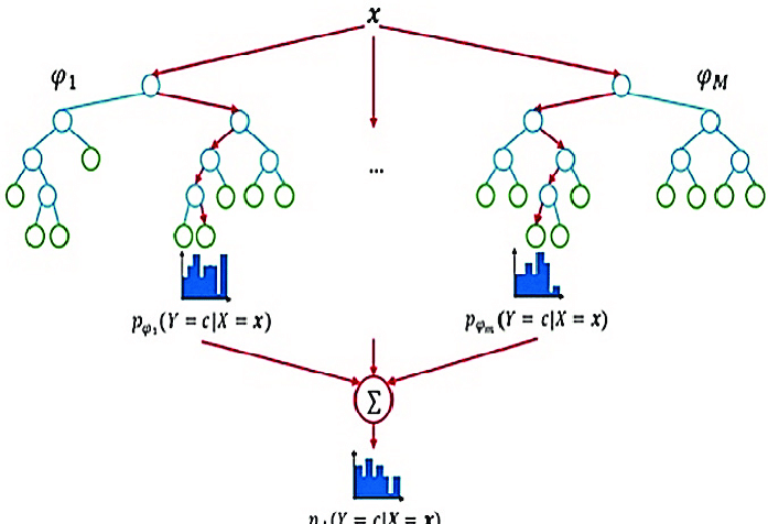
The following diagram will illustrate its working :

Algorithm:

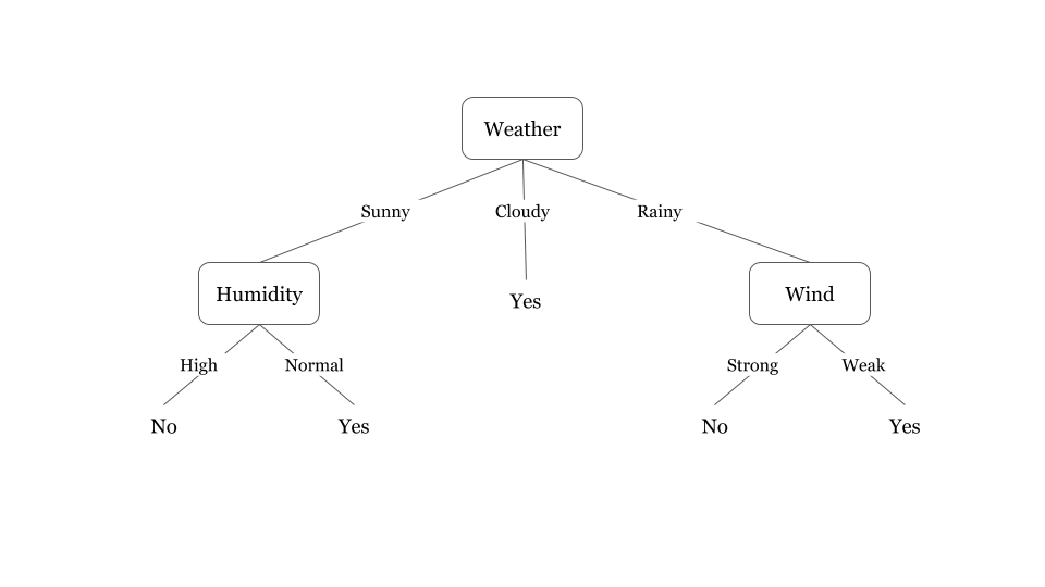
Preliminaries: decision tree learning

Decision trees are a popular method for various machine learning tasks. Tree learning “come[s] closest to meeting the requirements for serving as an off-the-shelf procedure for data mining”, say Hastie et al., “because it is invariant under scaling and various other transformations of feature values, is robust to inclusion of irrelevant features, and produces inspectable models. However, they are seldom accurate”.

In particular, trees that are grown very deep tend to learn highly irregular patterns: they overfit their training sets, i.e. have low bias, but very high variance. Random forests are a way of averaging multiple deep decision trees, trained on different parts of the same training set, with the goal of reducing the variance. This comes at the expense of a small increase in the bias and some loss of interpretability, but generally greatly boosts the performance in the final model.

Bagging:

The training algorithm for random forests applies the general technique of bootstrap aggregating, or bagging, to tree learners. Given a training set X = x1, …, xn with responses Y = y1, …, yn, bagging repeatedly (B times) selects a random sample with replacement of the training set and fits trees to these samples:

For b = 1, …, B:

Sample, with replacement, n training examples from X, Y; call these Xb, Yb.

Train a classification or regression tree fb on Xb, Yb.

After training, predictions for unseen samples x’ can be made by averaging the predictions from all the individual regression trees on x’:

From bagging to random forests

The above procedure describes the original bagging algorithm for trees. Random forests differ in only one way from this general scheme: they use a modified tree learning algorithm that selects, at each candidate split in the learning process, a random subset of the features. This process is sometimes called “feature bagging”. The reason for doing this is the correlation of the trees in an ordinary bootstrap sample: if one or a few features are very strong predictors for the response variable (target output), these features will be selected in many of the B trees, causing them to become correlated. An analysis of how bagging and random subspace projection contribute to accuracy gains under different conditions is given by Ho.

Typically, for a classification problem with p features, √p (rounded down) features are used in each split. For regression problems the inventors recommend p/3 (rounded down) with a minimum node size of 5 as the default.In practice the best values for these parameters will depend on the problem, and they should be treated as tuning parameters.

ExtraTrees:

Adding one further step of randomization yields extremely randomized trees, or ExtraTrees. While similar to ordinary random forests in that they are an ensemble of individual trees, there are two main differences: first, each tree is trained using the whole learning sample (rather than a bootstrap sample), and second, the top-down splitting in the tree learner is randomized. Instead of computing the locally optimal cut-point for each feature under consideration (based on, e.g., information gain or the Gini impurity), a random cut-point is selected. This value is selected from a uniform distribution within the feature’s empirical range (in the tree’s training set). Then, of all the randomly generated splits, the split that yields the highest score is chosen to split the node. Similar to ordinary random forests, the number of randomly selected features to be considered at each node can be specified. Default values for this parameter are {\displaystyle {\sqrt

Implementation in Python:

First, start with importing necessary Python packages :

Next, download the iris dataset from its web link as follows :

Next, we need to assign column names to the dataset as follows :

Now, we need to read dataset to pandas dataframe as follows :

sepal-length	sepal-width	petal-length	petal-width	Class
0	5.1	3.5	1.4	0.2	Iris-setosa
1	4.9	3.0	1.4	0.2	Iris-setosa
2	4.7	3.2	1.3	0.2	Iris-setosa
3	4.6	3.1	1.5	0.2	Iris-setosa
4	5.0	3.6	1.4	0.2	Iris-setosa

Data Preprocessing will be done with the help of following script lines.

X = dataset.iloc[:, :-1].values

y = dataset.iloc[:, 4].values

Next, we will divide the data into train and test split. The following code will split the dataset into 70% training data and 30% of testing data :

from sklearn.model_selection import train_test_split

X_train, X_test, y_train, y_test = train_test_split(X, y, test_size = 0.30)

Next, train the model with the help of RandomForestClassifier class of sklearn as follows :

Finally, we need to make predictions. It can be done with the help of following script y_pred = classifier.predict(X_test)

Next, print the results as follows :

Output

Confusion Matrix:

[[14 0 0]

[ 0 18 1]

[ 0 0 12]]

Classification Report:

	precision	recall	f1-score	support
Iris-setosa	1.00	1.00	1.00	14
Iris-versicolor	1.00	0.95	0.97	19
Iris-virginica	0.92	1.00	0.96	12

micro avg	0.98	0.98	0.98	45
macro avg	0.97	0.98	0.98	45
weighted avg	0.98	0.98	0.98	45

 Accuracy: 0.9777777777777777

Pros and Cons of Random Forest:

Pros:

The following are the advantages of Random Forest algorithm −

• It overcomes the problem of overfitting by averaging or combining the results of different decision trees.
• Random forests work well for a larger range of data items than a single decision tree does.
• Random forest has less variance than a single decision tree.
• Random forests are very flexible and possess very high accuracy.
• Scaling of data does not require a random forest algorithm. It maintains good accuracy even after providing data without scaling.
• Random Forest algorithms maintain good accuracy even if a large proportion of the data is missing.

Cons:

The following are the disadvantages of Random Forest algorithm −

• Complexity is the main disadvantage of Random forest algorithms.
• Construction of Random forests are much harder and time-consuming than decision trees.
• More computational resources are required to implement the Random Forest algorithm.
• It is less intuitive in case when we have a large collection of decision trees.
• The prediction process using random forests is very time-consuming in comparison with other algorithms.

Regression Algorithms – Overview:

Introduction to Regression :

Regression is another important and broadly used statistical and machine learning tool. The key objective of regression-based tasks is to predict output labels or responses which are continuous numeric values, for the given input data. The output will be based on what the model has learned in the training phase. Basically, regression models use the input data features (independent variables) and their corresponding continuous numeric output values (dependent or outcome variables) to learn specific associations between inputs and corresponding outputs.

Types of Regression Models:

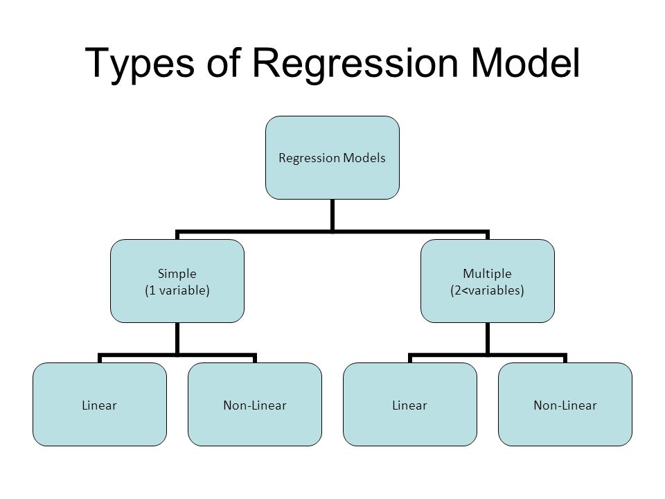
Regression models are of following two types :

• Simple regression model : This is the most basic regression model in which predictions are formed from a single, univariate feature of the data.
• Multiple regression model : As name implies, in this regression model the predictions are formed from multiple features of the data.
• Building a Regressor in Python: The Regressor model in Python can be constructed just like we constructed the classifier. Scikit-learn, a Python library for machine learning can also be used to build a regressor in Python.

In the following example, we will be building a basic regression model that will fit a line to the data i.e. linear regressor. The necessary steps for building a regressor in Python are as follows −

Step 1: Importing necessary python package

For building a regression using scikit-learn, we need to import it along with other necessary packages. We can import the by using following script :

Step 2: Importing dataset

After importing the necessary package, we need a dataset to build a regression prediction model. We can import it from a sklearn dataset or can use another one as per our requirement. We are going to use our saved input data. We can import it with the help of following script :

• input = r’C:\linear.txt’
• Next, we need to load this data. We are using np.loadtxt function to load it.
• input_data = np.loadtxt(input, delimiter=’,’)
• X, y = input_data[:, :-1], input_data[:, -1]

Step 3: Organizing data into training & testing sets

As we need to test our model on unseen data hence, we will divide our dataset into two parts: a training set and a test set. The following command will perform it.

Step 4: Model evaluation & prediction

After dividing the data into training and testing we need to build the model. We will be using LineaRegression() function of Scikit-learn for this purpose. Following command will create a linear regression object.

Step 5: Plot & visualization

plt.show()

Output :



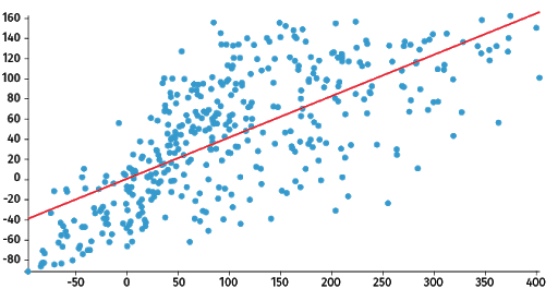
In the above output, we can see the regression line between the data points.

Step 6: Performance computation : We can also compute the performance of our regression model with the help of various performance metrics as follows.

Random Forest Sample Resumes! Download & Edit, Get Noticed by Top Employers! Download

Unsupervised learning with Random forests:

As part of their construction, random forest predictors naturally lead to a dissimilarity measure among the observations. One can also define a random forest dissimilarity measure between unlabeled data: the idea is to construct a random forest predictor that distinguishes the “observed” data from suitably generated synthetic data. The observed data are the original unlabeled data and the synthetic data are drawn from a reference distribution. A random forest dissimilarity can be attractive because it handles mixed variable types very well, is invariant to monotonic transformations of the input variables, and is robust to outlying observations. The random forest dissimilarity easily deals with a large number of semi-continuous variables due to its intrinsic variable selection; for example, the “Addcl 1” random forest dissimilarity weighs the contribution of each variable according to how dependent it is on other variables. The random forest dissimilarity has been used in a variety of applications, e.g. to find clusters of patients based on tissue marker data.

Conclusion: Random Forest is a great algorithm, for both classification and regression problems, to produce a predictive model. Its default hyperparameters already return great results and the system is great at avoiding overfitting. Moreover, it is a pretty good indicator of the importance it assigns to your features.