
Last updated on 07th Jul 2020| 2372
Naive Bayes
Naive Bayes is among one of the most simple and powerful algorithms for classification based on Bayes’ Theorem with an assumption of independence among predictors. Naive Bayes model is easy to build and particularly useful for very large data sets. There are two parts to this algorithm:
- Naive
- Bayes
The Naive Bayes classifier assumes that the presence of a feature in a class is unrelated to any other feature. Even if these features depend on each other or upon the existence of the other features, all of these properties independently contribute to the probability that a particular fruit is an apple or an orange or a banana and that is why it is known as “Naive”.
Mathematics of Probability required
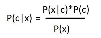
The Bayes theorem’s equation:
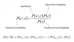
- P(c|x) = P(c and x)/ P(x)
- P(c|x) is the posterior probability of class (c, target) given predictor (x, attributes).
- P(c) is the prior probability of class.
- P(x|c) is the likelihood which is the probability of predictor given class.
- P(x) is the prior probability of predictor.
In Naive Bayes all we want to find is the posterior probability values. The posterior probability value for whichever class is highest will be the final result of the problem we solve.
Bayes’ Theorem is useful for dealing with conditional probabilities, since it provides a way for us to reverse them.
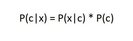
Here we can simply ignore the denominator which is predictor prior probability or some refer to it as evidence probability, because for whatever the problem consisting of many target variables , the probability of that would be same for all the classes. After ignoring the denominators we are simply left with this equation,
4 Applications of Naive Bayes Algorithms
- Real time Prediction: Naive Bayes is an eager learning classifier and it is sure fast. Thus, it could be used for making predictions in real time.
- Multi class Prediction: This algorithm is also well known for multi class prediction feature. Here we can predict the probability of multiple classes of target variable.
- Text classification/ Spam Filtering/ Sentiment Analysis: Naive Bayes classifiers mostly used in text classification (due to better result in multi class problems and independence rule) have higher success rate as compared to other algorithms. As a result, it is widely used in Spam filtering (identify spam e-mail) and Sentiment Analysis (in social media analysis, to identify positive and negative customer sentiments)
- Recommendation System: Naive Bayes Classifier and Collaborative Filtering together builds a Recommendation System that uses machine learning and data mining techniques to filter unseen information and predict whether a user would like a given resource or not
Naive Bayes Used
You can use Naive Bayes for the following things:
- Face Recognition
- As a classifier, it is used to identify the faces or its other features, like nose, mouth, eyes, etc.
- Weather Prediction
- It can be used to predict if the weather will be good or bad.
- Medical Diagnosis
Doctors can diagnose patients by using the information that the classifier provides. Healthcare professionals can use Naive Bayes to indicate if a patient is at high risk for certain diseases and conditions, such as heart disease, cancer, and other ailments.
News Classification
With the help of a Naive Bayes classifier, Google News recognizes whether the news is political, world news, and so on.
As the Naive Bayes Classifier has so many applications, it’s worth learning more about how it works.
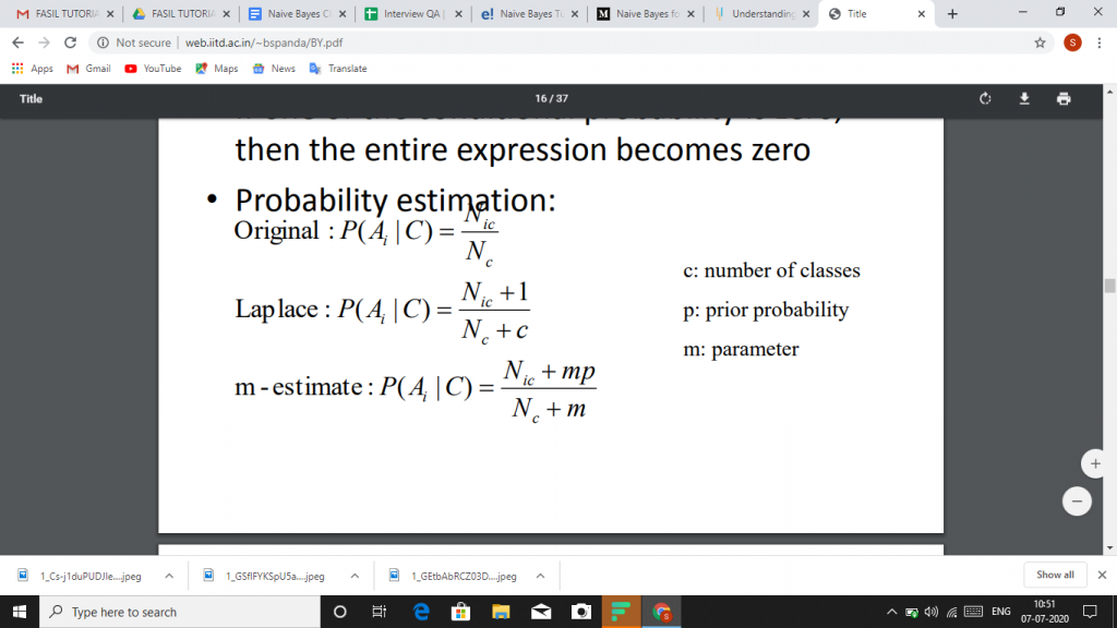
Naïve Bayes Classifier
- If one of the conditional probability is zero, then the entire expression becomes zero
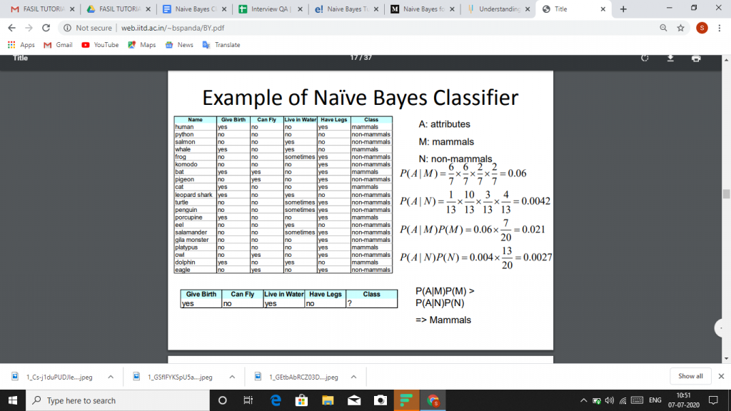
Naive Bayes classifier works
Let’s understand the working of Naive Bayes through an example. Given an example of weather conditions and playing sports. You need to calculate the probability of playing sports. Now, you need to classify whether players will play or not, based on the weather condition.

Get JOB Oriented Machine Learning Training for Beginners By Industry Experts
- Instructor-led Sessions
- Real-life Case Studies
- Assignments
First Approach (In case of a single feature)
Naive Bayes classifier calculates the probability of an event in the following steps:
- Step 1: Calculate the prior probability for given class labels
- Step 2: Find Likelihood probability with each attribute for each class
- Step 3: Put these value in Bayes Formula and calculate posterior probability.
- Step 4: See which class has a higher probability, given the input belongs to the higher probability class.
For simplifying prior and posterior probability calculation you can use the two tables frequency and likelihood tables. Both of these tables will help you to calculate the prior and posterior probability. The Frequency table contains the occurrence of labels for all features. There are two likelihood tables. Likelihood Table 1 is showing prior probabilities of labels and Likelihood Table 2 is showing the posterior probability.
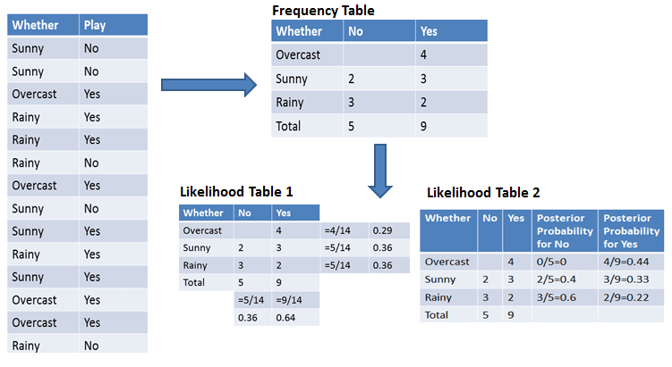
Now suppose you want to calculate the probability of playing when the weather is overcast.
Probability of playing:
P(Yes | Overcast) = P(Overcast | Yes) P(Yes) / P (Overcast) …………………(1)
- Calculate Prior Probabilities:P(Overcast) = 4/14 = 0.29P(Yes)= 9/14 = 0.64
- Calculate Posterior Probabilities:P(Overcast |Yes) = 4/9 = 0.44
- Put Prior and Posterior probabilities in equation (1)P (Yes | Overcast) = 0.44 * 0.64 / 0.29 = 0.98(Higher)
Similarly, you can calculate the probability of not playing:
Probability of not playing:
P(No | Overcast) = P(Overcast | No) P(No) / P (Overcast) …………………(2)
- Calculate Prior Probabilities:P(Overcast) = 4/14 = 0.29P(No)= 5/14 = 0.36
- Calculate Posterior Probabilities:P(Overcast |No) = 0/9 = 0
- Put Prior and Posterior probabilities in equation (2)P (No | Overcast) = 0 * 0.36 / 0.29 = 0
Classifier Building in Scikit-learn
Naive Bayes Classifier
Defining Dataset
In this example, you can use the dummy dataset with three columns: weather, temperature, and play. The first two are features(weather, temperature) and the other is the label.
- # Assigning features and label variables
- weather=[‘Sunny’,’Sunny’,’Overcast’,’Rainy’,’Rainy’,’Rainy’,’Overcast’,’Sunny’,’Sunny’,
- ‘Rainy’,’Sunny’,’Overcast’,’Overcast’,’Rainy’]
- temp=[‘Hot’,’Hot’,’Hot’,’Mild’,’Cool’,’Cool’,’Cool’,’Mild’,’Cool’,’Mild’,’Mild’,’Mild’,’Hot’,’Mild’]
- play=[‘No’,’No’,’Yes’,’Yes’,’Yes’,’No’,’Yes’,’No’,’Yes’,’Yes’,’Yes’,’Yes’,’Yes’,’No’]
Encoding Features
First, you need to convert these string labels into numbers. for example: ‘Overcast’, ‘Rainy’, ‘Sunny’ as 0, 1, 2. This is known as label encoding. Scikit-learn provides LabelEncoder library for encoding labels with a value between 0 and one less than the number of discrete classes.
- # Import LabelEncoder from sklearn import preprocessing
- #creating labelEncoder
- le = preprocessing.LabelEncoder()
- # Converting string labels into numbers.
- wheather_encoded=le.fit_transform(wheather)
- print wheather_encoded
- [2 2 0 1 1 1 0 2 2 1 2 0 0 1]
Similarly, you can also encode temp and play columns.
- # Converting string labels into numbers
- temp_encoded=le.fit_transform(temp)
- label=le.fit_transform(play)
- print “Temp:”,temp_encoded
- print “Play:”,label
- Temp: [1 1 1 2 0 0 0 2 0 2 2 2 1 2]
- Play: [0 0 1 1 1 0 1 0 1 1 1 1 1 0]
Now combine both the features (weather and temp) in a single variable (list of tuples).
- #Combinig weather and temp into single listof tuples
- features=zip(weather_encoded,temp_encoded)
- print features
- [(2, 1), (2, 1), (0, 1), (1, 2), (1, 0), (1, 0), (0, 0), (2, 2), (2, 0), (1, 2), (2, 2), (0, 2), (0, 1)]
Generating Model
Generate a model using naive bayes classifier in the following steps:
- Create naive bayes classifier
- Fit the dataset on classifier
- Perform prediction
- #Import Gaussian Naive Bayes model
- from sklearn.naive_bayes import GaussianNB
- #Create a Gaussian Classifier
- model = GaussianNB()
- # Train the model using the training sets
- model.fit(features,label)
- #Predict Output
- predicted= model.predict([[0,2]]) # 0:Overcast, 2:Mild
- print “Predicted Value:”, predicted
- Predicted Value: [1]
Naive Bayes with Multiple Labels
Till now you have learned Naive Bayes classification with binary labels. Now you will learn about multiple class classification in Naive Bayes. Which is known as multinomial Naive Bayes classification. For example, if you want to classify a news article about technology, entertainment, politics, or sports.
In model building part, you can use wine dataset which is a very famous multi-class classification problem. “This dataset is the result of a chemical analysis of wines grown in the same region in Italy but derived from three different cultivars.” (UC Irvine)
Dataset comprises of 13 features (alcohol, malic_acid, ash, alcalinity_of_ash, magnesium, total_phenols, flavanoids, nonflavanoid_phenols, proanthocyanins, color_intensity, hue, od280/od315_of_diluted_wines, proline) and type of wine cultivar. This data has three type of wine Class_0, Class_1, and Class_3. Here you can build a model to classify the type of wine.
The dataset is available in the scikit-learn library.
Loading Data
Let’s first load the required wine dataset from scikit-learn datasets.
- #Import scikit-learn dataset library from sklearn import datasets
- #Load dataset
- wine = datasets.load_wine()
Exploring Data
You can print the target and feature names, to make sure you have the right dataset, as such:
- # print the names of the 13 features
- print “Features: “, wine.feature_names
- # print the label type of wine(class_0, class_1, class_2)
- print “Labels: “, wine.target_names
- Features: [‘alcohol’, ‘malic_acid’, ‘ash’, ‘alcalinity_of_ash’, ‘magnesium’, ‘total_phenols’, ‘flavanoids’, ‘nonflavanoid_phenols’, ‘proanthocyanins’, ‘color_intensity’, ‘hue’, ‘od280/od315_of_diluted_wines’, ‘proline’]
- Labels: [‘class_0’ ‘class_1’ ‘class_2’]
It’s a good idea to always explore your data a bit, so you know what you’re working with. Here, you can see the first five rows of the dataset are printed, as well as the target variable for the whole dataset.
- # print data(feature)shape
- wine.data.shape
- (178L, 13L)
- # print the wine data features (top 5 records)
- print wine.data[0:5]
- [[ 1.42300000e+01 1.71000000e+00 2.43000000e+00 1.56000000e+01 1.27000000e+02 2.80000000e+00 3.06000000e+00 2.80000000e-01 2.29000000e+00 5.64000000e+00 1.04000000e+00 3.92000000e+00 1.06500000e+03]
- [ 1.32000000e+01 1.78000000e+00 2.14000000e+00 1.12000000e+01 1.00000000e+02 2.65000000e+00 2.76000000e+00 2.60000000e-01 1.28000000e+00 4.38000000e+00 1.05000000e+00 3.40000000e+00 1.05000000e+03]
- [ 1.31600000e+01 2.36000000e+00 2.67000000e+00 1.86000000e+01 1.01000000e+02 2.80000000e+00 3.24000000e+00 3.00000000e-01 2.81000000e+00 5.68000000e+00 1.03000000e+00 3.17000000e+00 1.18500000e+03]
- [ 1.43700000e+01 1.95000000e+00 2.50000000e+00 1.68000000e+01 1.13000000e+02 3.85000000e+00 3.49000000e+00 2.40000000e-01 2.18000000e+00 7.80000000e+00 8.60000000e-01 3.45000000e+00 1.48000000e+03]
- [ 1.32400000e+01 2.59000000e+00 2.87000000e+00 2.10000000e+01 1.18000000e+02 2.80000000e+00 2.69000000e+00 3.90000000e-01 1.82000000e+00 4.32000000e+00 1.04000000e+00 2.93000000e+00 7.35000000e+02]]
- # print the wine labels (0:Class_0, 1:class_2, 2:class_2)
- print wine.target
- [0 0 0 0 0 0 0 0 0 0 0 0 0 0 0 0 0 0 0 0 0 0 0 0 0 0 0 0 0 0 0 0 0 0 0 0 0 0 0 0 0 0 0 0 0 0 0 0 0 0 0 0 0 0 0 0 0 0 0 1 1 1 1 1 1 1 1 1 1 1 1 1 1 1 1 1 1 1 1 1 1 1 1 1 1 1 1 1 1 1 1 1 1 1 1 1 1 1 1 1 1 1 1 1 1 1 1 1 1 1 1 1 1 1 1 1 1 1 1 1 1 1 1 1 1 1 1 1 1 1 2 2 2 2 2 2 2 2 2 2 2 2 2 2 2 2 2 2 2 2 2 2 2 2 2 2 2 2 2 2 2 2 2 2 2 2 2 2 2 2 2 2 2 2 2 2 2 2]
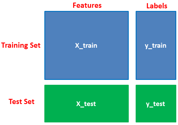
Splitting Data
First, you separate the columns into dependent and independent variables(or features and label). Then you split those variables into train and test set.
- # Import train_test_split function
- from sklearn.cross_validation import train_test_split
- # Split dataset into training set and test set
- X_train, X_test, y_train, y_test = train_test_split(wine.data, wine.target, test_size=0.3,random_state=109)
- # 70% training and 30% test
Model Generation
After splitting, you will generate a random forest model on the training set and perform prediction on test set features.
- #Import Gaussian Naive Bayes model
- from sklearn.naive_bayes import GaussianNB
- #Create a Gaussian Classifier
- gnb = GaussianNB()
- #Train the model using the training sets
- gnb.fit(X_train, y_train)
- #Predict the response for test dataset
- y_pred = gnb.predict(X_test)
Evaluating Model
After model generation, check the accuracy using actual and predicted values.
- #Import scikit-learn metrics module for accuracy calculation
- from sklearn import metrics
- # Model Accuracy, how often is the classifier correct?
- print(“Accuracy:”,metrics.accuracy_score(y_test, y_pred))
- (‘Accuracy:’, 0.90740740740740744)
Advantages
- It is not only a simple approach but also a fast and accurate method for prediction.
- Naive Bayes has very low computation cost.
- It can efficiently work on a large dataset.
- It performs well in case of discrete response variable compared to the continuous variable.
- It can be used with multiple class prediction problems.
- It also performs well in the case of text analytics problems.
- When the assumption of independence holds, a Naive Bayes classifier performs better compared to other models like logistic regression.
Conclusion
In this tutorial, you learned about Naïve Bayes algorithm, it’s working, Naive Bayes assumption, issues, implementation, advantages. Along the road, you have also learned model building and evaluation in scikit-learn for binary and multinomial classes.
Naive Bayes is the most straightforward and most potent algorithm. In spite of the significant advances of Machine Learning in the last couple of years, it has proved its worth. It has been successfully deployed in many applications from text analytics to recommendation engines.