Tutorial on Statistics and Probability for Data Science | All you need to know [ OverView ]

Last updated on 11th Jan 2022, Blog, Tutorials

• Introduction to Statistics and Probability
• What is Data?
• Categories Of Data
• What is Statistics?
• Basic Terminologies In Statistics
• Types Of Statistics
• Understanding Descriptive Statistics
• What is Probability
• Terminologies In Probability
• Probability Distribution
• Types Of Probability
• Joint Probability
• Statistical Inference
• Conclusion

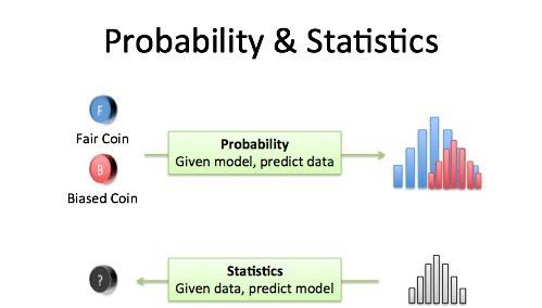
Introduction to Statistics and Probability:

Statistics and chance are the building blocks of the foremost revolutionary technologies in today’s world. From computer science to Machine Learning and pc Vision, Statistics and chance kind the fundamental foundation to all or any such technologies. During this article on Statistics and chance, I will assist you to perceive the math behind the foremost complicated algorithms and technologies.

To get in-depth knowledge on Data Science and the various Machine Learning Algorithms, you can enroll for live Data Science Certification Training by ACTE with 24/7 support and lifetime access.

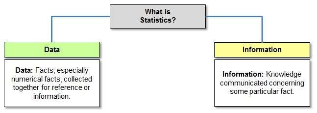
What is Data?

• Look around you, there’s knowledge all over. every click on your phone generates a lot more knowledge than you recognize. This generated knowledge provides insights for analysis and helps the United States build higher business selections. This is often why knowledge is thus vital.
• Data refers to facts and statistics collected along for reference or analysis.
• Data will be collected, measured and analyzed. It may be envisioned by using applied math models and graphs.

Categories Of Data:

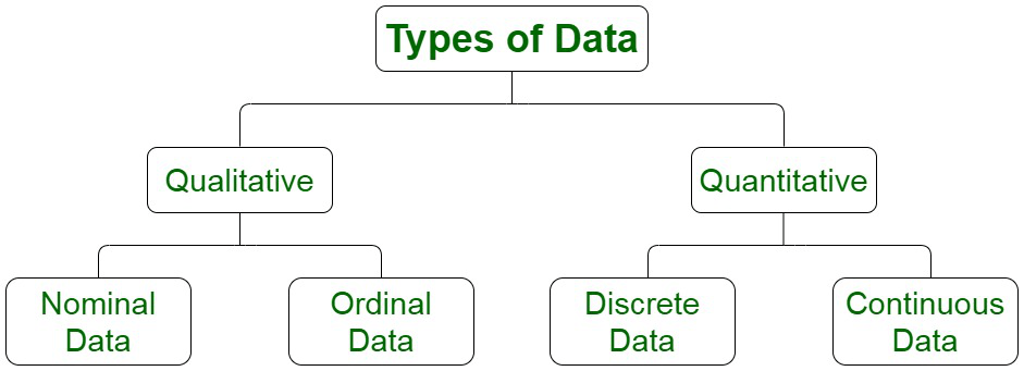
Data will be classified into 2 sub-categories:

• Qualitative data
• Quantitative data

Refer the below figure to grasp the various classes of data:

Qualitative Data: Qualitative data deals with characteristics and descriptors that can’t be simply measured, however will be determined subjectively. Qualitative data is more divided into 2 styles of data:

Nominal data: Data with no inherent order or ranking like gender or race.

Nominal data Statistics and likelihood – ACTE

Ordinal data: Data with an measure of data is termed ordinal data.

Quantitative Data: Quantitative data deals with numbers and stuff you will live objectively. this can be more divided into two:

Discrete Data: Additionally referred to as categorical data, it will hold a finite variety of attainable values.

Example: variety of scholars during a category.

Continuous data: Data that may hold an infinite variety of attainable values.

Example: Weight of an individual.

So these were the various classes of knowledge. The future sections can concentrate on the essential Statistics ideas, thus buckle up and find able to do some math.

What is Statistics?

Statistics is a neighborhood of applied math involved with data assortment, analysis, interpretation, and presentation

This space of arithmetic deals with understanding however data is often accustomed to solve advanced issues. Here area unit a handful of example issues that may be resolved by exploitation statistics:

• Your company has created a replacement drug which will cure cancer. however would you conduct a check to substantiate the drug’s effectiveness?
• You and a lover area unit at a baseball game, and out of the blue, he offers you a bet that neither team can hit a home run therein game. must you take the bet? The latest sales data is simply available, and your boss needs you to organize a report for management on places wherever the corporation may improve its business. What must you look for? What must you not look for?
• These preceding issues are often simply resolved by exploitation applied mathematics techniques. within the approaching sections, we’ll see however this will be done.
• If you wish an additional in-depth rationalization on Statistics and chance, you’ll be able to check up on this video by our Statistics specialists.

Basic Terminologies In Statistics:

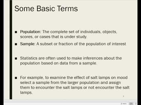
Before you dive deep into Statistics, it’s necessary that you just perceive the fundamental terminologies employed in Statistics. The 2 most vital terminologies in statistics are population and sample.

Population: a group or set of people or objects or events whose properties are to be analyzed.

Sample: A set of the population is termed ‘Sample’. A happy sample can contain most of the knowledge a couple of specific population parameter. Now you want to be questioning however one will opt for a sample that best represents the whole population.

Sampling Techniques:

Sampling may be a method that deals with the choice of individual observations among a population. it’s performed to infer applied mathematics data a couple of population.

Consider a situation whereby you’re asked to perform a survey concerning the uptake habits of teenagers within the USA. Their are over forty two million teens within the USA nowadays and this range is growing as you browse this diary. is it potential to survey every of those forty two million people concerning their health? clearly not! That’s why sampling is employed. it’s a way whereby a sample of the population is studied so as to draw illation concerning the whole population.

There are 2 main styles of Sampling techniques:

• Probability Sampling
• Non-Probability Sampling

In this diary, we’ll be focusing solely on likelihood sampling techniques as a result of non-probability sampling isn’t among the scope of this diary.

Probability Sampling: this can be a sampling technique during which samples from an outsized population are chosen using the speculation of likelihood. There are 3 styles of likelihood sampling:

Random Sampling: During this methodology, every member of the population has AN equal probability of being elite within the sample.

Systematic Sampling: In Systematic sampling, each ordinal record is chosen from the population to be a region of the sample. Refer the below figure to raise perception however Systematic sampling works.

Stratified Sampling: In representative sampling, a stratum is employed to make samples from an outsized population. A stratum may be a set of the population that shares a minimum of one common characteristic. After this, the sampling methodology is employed to pick a sufficient range of subjects from every stratum. Now that you just grasp the fundamentals of Statistics, let’s move ahead and discuss the various styles of statistics.

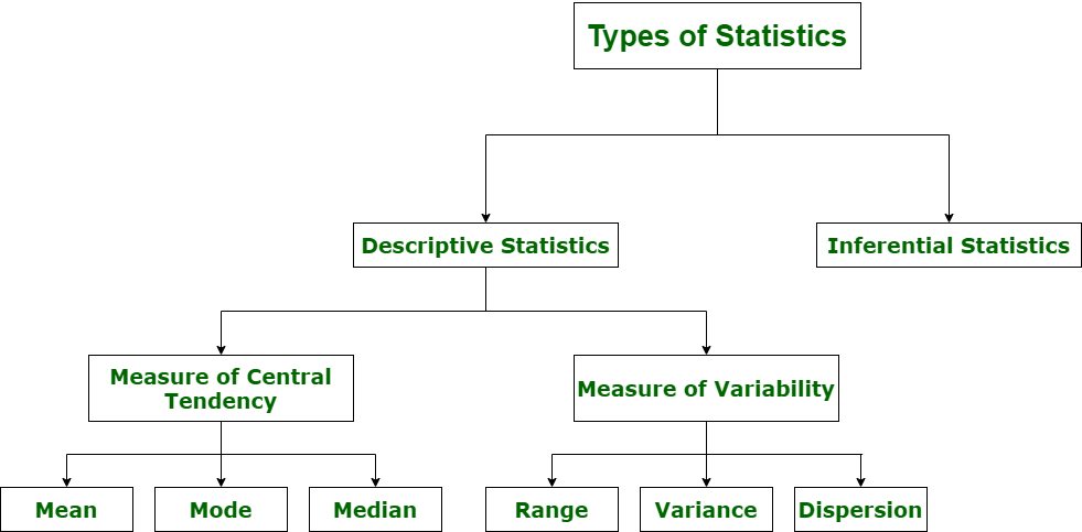
Types Of Statistics:

There are 2 well-defined sorts of statistics:

• Descriptive Statistics
• Inferential Statistics

Descriptive Statistics

Descriptive statistics could be a technique used to describe and perceive the options of a selected data set by giving short summaries concerning the sample and measures of the info.

Descriptive Statistics is especially targeted upon the most characteristics of knowledge. It provides a graphical outline of the info. Suppose you wish to administer all of your classmate’s t-shirts. to review the typical shirt size of scholars in an exceedingly room, in descriptive statistics you’d record the shirt size of all students within the category so you’d decide the utmost, minimum and average shirt size of the category.

Inferential Statistics

Inferential statistics makes inferences and predictions a few populations supported a sample of knowledge taken from the population in question. Inferential statistics generalizes an oversized dataset and applies a chance to draw a conclusion. It permits the United States to infer data parameters supporting an applied mathematics model using sample data.

So, if we tend to take into account constant examples of finding the typical shirt size of scholars in an exceedingly large category, in Inferential Statistics, you’ll take a sample set of the category, that is essentially a couple of individuals from the complete category. You have already classified the category into massive, medium and tiny. During this technique, you primarily build an applied mathematics model and expand it for the complete population within the category.

So that was a short understanding of Descriptive and Inferential Statistics. within any sections, you’ll see however Descriptive and Inferential statistics works comprehensively.

Understanding Descriptive Statistics:

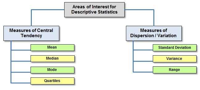
Descriptive Statistics is diminished into 2 categories:

• Measures of Central Tendency
• Measures of Variability (spread)

Measures Of Center

Measures of the center area unit applied math measures that represent the outline of a dataset. There area unit 3 main measures of center:

Mean: live of the typical of all the values in an exceedingly sample is termed Mean.

Median: live of the central price of the sample set is termed Median.

Mode: the worth most repeated within the sample set is thought as Mode.

To better perceive the Measures of central tendency let’s inspect associate degree examples. The below cars dataset contains the subsequent variables:

Quartile: Quartiles tell America concerning the unfold of an data set by breaking the data set into quarters, rather like the median breaks it in [*fr1].

• To better perceive however grade and also the IQR area unit calculated, let’s inspect associate degree example
• The higher than image shows marks of a hundred students ordered from lowest to highest scores. The quartiles dwell the subsequent ranges.
• The first grade (Q1) lies between the twenty fifth and twenty sixth observations.
• The second grade (Q2) lies between the fiftieth and 51st observation.
• The third grade (Q3) lies between the seventy fifth and 76th observation.
• InterQuartile vary (IQR): it’s the life of variability, supported dividing an data set into quartiles. The interquartile vary is up to Q3 minus Q1, i.e. IQR = Q3 – Q1

Variance: It describes what quantity a stochastic variable differs from its mean. It entails computing squares of deviations. Variance will be calculated by mistreatment the below formula:

Let’s inspect the answer step by step:

Step 1: determine the mean for your sample set.

Step 2: Then for every variety, take off the Mean and sq. the result.

Step 3: Then estimate the mean of these square variations.

To better perceive the measures of unfold and centre, let’s execute a brief demo by exploiting the R language.

Descriptive Statistics In R:

R could be an applied math artificial language that’s in the main used for knowledge Science, Machine Learning then on. If you would like to find out a lot regarding R, offer this R Tutorial – A Beginner’s Guide to find out R Programming journal a browse. Now let’s move ahead and implement Descriptive Statistics in R.

In this demo, we’ll see a way to calculate the Mean, Median, Mode, Variance, variance and the way to check the variables by plotting a bar graph. This is often quite an easy demo however it conjointly forms the muse that each Machine Learning formula is made upon.

Problem Statement: To predict whether or not a match may be vie or not by finding out the climatic conditions.

Data Set Description: the subsequent knowledge set contains observations regarding the climatic conditions over an amount of your time.

What is Probability:

Probability is that the life of however possible an occasion can occur. To be a lot of precise chance is that the magnitude relation of desired outcomes to total outcomes:

The probabilities of all outcomes invariably sums up to one. think about the illustrious rolling dice example:

• On rolling a dice, you get half-dozen potential outcomes
• Each chance solely has one outcome, thus every features a chance of 1/6
• For example, the chance of obtaining variety ‘2’ on the dice is 1/6
• Now let’s try and perceive the common terminologies employed by chance.

Terminologies In Probability:

Before you dive deep into the ideas of chance, it’s vital that you simply perceive the essential terminologies employed in probability:

Random Experiment: AN experiment or a method that the result can’t be expected with certainty.

Sample area: the whole potential set of outcomes of a random experiment is the sample space of that experiment.

Event: One or a lot of outcomes of AN experiment is called an occasion. It’s a set of sample areas. There are 2 sorts of events in probability:

Disjoint Event: Disjoint Events don’t have any common outcomes. for instance, one card drawn from a deck can’t be a king and a queen

Non – Disjoint Event: Non-Disjoint Events will have common outcomes. for instance, a student will get a hundred marks in statistics and a hundred marks in chance

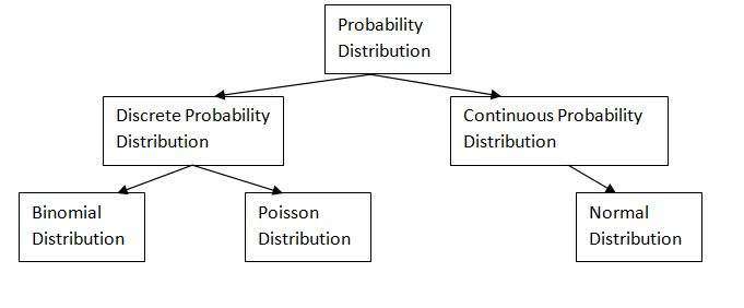
Probability Distribution:

In this diary we have a tendency to shall target 3 main likelihood distribution functions:

• Probability Density operate
• Normal Distribution
• Central Limit Theorem
• Probability Density operate

The likelihood Density operate (PDF) worries with the relative chance for a nonstop variate to require on a given price. The PDF provides the likelihood of a variable that lies between the vary ‘a’ and ‘b’.

Types Of Probability:

Marginal likelihood

The likelihood of an incident occurring (p(A)), unconditioned on the other events. as an example, the likelihood that a card drawn may be a three (p(three)=1/13).

Central Limit Theorem

• The Central Limit Theorem states that the sampling distribution of the mean of any freelance, variant are going to be traditional or nearly traditional if the sample size is massive enough.
• In easy terms, if we tend to have an outsized population divided into samples, then the mean of all the samples from the population would be nearly up to the mean of the complete population. The below graph depicts a a lot of clear understanding of the Central Limit Theorem.



The accuracy or alikeness to the traditional distribution depends on 2 main factors:

• Number of sample points taken
• The shape of the underlying population
• Now let’s specialize in the 3 main styles of likelihood.

Joint Probability:

Joint Probability could be a life of 2 events happening at an equivalent time, i.e., p(A and B), The likelihood of event A and event B occurring. it’s the likelihood of the intersection of 2 or a lot of events. The likelihood of the intersection of A and B is also written p(A ∩ B).

For example, the likelihood that a card could be a four and red =p(four and red) = 2/52=1/26.

Conditional likelihood:

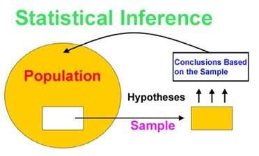
Statistical Inference:

As mentioned earlier, applied math logical thinking could be a branch of statistics that deals with forming inferences and predictions. A couple of populations supported a sample of data taken from the population in question. The question you ought to raise currently, is however do you kind inferences or predictions on a sample? The solution is thru purpose estimation.

What is the purpose of Estimation?

Point Estimation cares with the utilization of the sample data to live one price that is Associate in Nursing approximate price or the most effective estimate of Associate in Nursing unknown population parameter.

Two necessary terminologies on purpose Estimation are:

Estimator: A performs f(x) of the sample, that’s want to conclude the estimate.

Estimate: The realized price of Associate in Nursing figure.

For example, so as to calculate the mean of an enormous population, we tend to 1st put off a sample of the population and notice the sample mean. The sample mean is then wont to estimate the population mean. this can be primarily purpose estimation.

Finding The Estimates:

There are four common applied math techniques that are wont to notice the calculable price involved with a population:

Method of Moments: it’s a way to estimate population parameters, just like the population mean or the population variance. In easy terms this involves, taking down proverbial facts regarding the population, and increasing those ideas to a sample.

Maximum of Likelihood: This technique uses a model and also the values within the model to maximize a chance to perform. This ends up in the foremost doubtless parameter for the inputs elite.

Bayes’ Estimators: This technique works by minimizing the typical risk (an expectation of random variables).

Best Unbiased Estimators: During this technique, many unbiased estimators are often wont to approximate a parameter (which one is “best” depends on what.

Conclusion:

Probability denotes the possibility of the outcome of any random event. The meaning of this term is to check the extent to which any event is likely to happen. For example, when we flip a coin in the air, what is the possibility of getting a head? The answer to this question is based on the number of possible outcomes. Here the possibility is either head or tail will be the outcome. So, the probability of a head to come as a result is 1/2.

The probability is the measure of the likelihood of an event to happen. It measures the certainty of the event. The formula for probability is given by:

Statistics is the study of the collection, analysis, interpretation, presentation, and organisation of data. It is a method of collecting and summarising the data. This has many applications from a small scale to large scale. Whether it is the study of the population of the country or its economy, stats are used for all such data analysis. Statistics has a huge scope in many fields such as sociology, psychology, geology, weather forecasting, etc. The data collected here for analysis could be quantitative or qualitative. Quantitative data are also of two types such as: discrete and continuous. Discrete data has a fixed value whereas continuous data is not a fixed data but has a range. There are many terms and formulas used in this concept.