Naive Bayes Theorem Explained: From Basics to Real-World Applications

Bayes’ Theorem Refresher

Text classification is one of the most effective domains for Naive Bayes. Machine Learning Training: The model treats each word in a document as an independent feature and uses word frequencies or presence to calculate probabilities.

For a document ( D ) and class ( C ):

• P(C|D) \propto P(C) \prod_{i=1}^{n} P(w_i|C)
• where ( w_i ) represents individual words.

Common examples include:

Spam filtering: Detecting spam based on the probability of certain words like “win”, “free”, or “offer”.

Sentiment analysis: Determining whether a review is positive or negative based on word patterns.

Topic classification: Categorizing articles into domains such as politics, sports, or technology.

Despite newer deep learning approaches, Naive Bayes remains competitive for large text corpora due to its simplicity and interpretability.

Subscribe To Contact Course Advisor

Subscribe

Understanding the Naive Bayes Classifier

Naive Bayes applies Bayes’ Theorem with one simplifying assumption: all features are conditionally independent given the class label. In other words, the presence or value of one feature does not influence another when the class is known. This assumption might seem unrealistic — for instance, in a spam detection task, the words “free” and “win” often appear together — but it allows the model to simplify calculations dramatically. Despite the simplification, the algorithm often produces surprisingly accurate results.



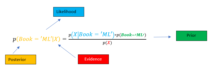
The general formula for Naive Bayes classification is:

• P(Y|X_1, X_2, …, X_n) \propto P(Y) \prod_{i=1}^{n} P(X_i|Y)

Here, ( Y ) represents the class (for example, spam or not spam), and ( X_1, X_2, …, X_n ) are the features (like words or numerical values). The class with the highest posterior probability becomes the model’s prediction. Naive Bayes classifiers are especially efficient when dealing with large datasets because they require only a small amount of training data to estimate parameters. This makes them ideal for real-time or resource-constrained systems.




Ready to Get Certified in Machine Learning? Explore the Program Now Machine Learning Online Training Offered By ACTE Right Now!




Assumptions of Naive Bayes

The power of Naive Bayes lies in its simplicity, but that simplicity comes from certain assumptions:

• Conditional Independence: All features are assumed independent given the class label.
• Equal Feature Importance: Each feature contributes equally to determining the class.
• Representative Data: Training data accurately reflects the underlying distribution of future data.

In practice, these assumptions rarely hold perfectly, but the classifier still performs well because classification depends more on the relative ranking of probabilities than on their exact values.




Types of Naive Bayes Classifiers

There are three main types of Naive Bayes models, each adapted to specific data characteristics. Gaussian Naive Bayes Used when features are continuous and assumed to follow a normal (Gaussian) distribution.

• For a feature ( x ) with mean ( \mu ) and variance ( \sigma^2 ) for a particular class ( Y ):
• P(x|Y) = \frac{1}{\sqrt{2\pi\sigma^2}} \exp\left( -\frac{(x – \mu)^2}{2\sigma^2} \right)

This form is popular in datasets like the Iris flower dataset, where features such as petal width or length are continuous measurements.

Multinomial Naive Bayes

Best suited for count data, such as the number of times a word appears in a document. It assumes features represent the frequency of discrete events. It’s heavily used in text classification, such as detecting spam or categorizing news articles.

Bernoulli Naive Bayes

Handles binary/Boolean features, representing whether a word or feature is present (1) or absent (0). This model is ideal for document classification tasks using binary word occurrence data.

Each variant modifies the likelihood estimation to match the data distribution, but the underlying Bayesian reasoning remains consistent.




Naive Bayes in Text Classification

Text classification is one of the most effective domains for Naive Bayes. The model treats each word in a document as an independent feature and uses word frequencies or presence to calculate probabilities.

For a document ( D ) and class ( C ):

• P(C|D) \propto P(C) \prod_{i=1}^{n} P(w_i|C)
• where ( w_i ) represents individual words.

Common examples include:

Spam filtering: Detecting spam based on the probability of certain words like “win”, “free”, or “offer”.

• Sentiment analysis: Determining whether a review is positive or negative based on word patterns.
• Topic classification: Categorizing articles into domains such as politics, sports, or technology.

Despite newer deep learning approaches, Naive Bayes remains competitive for large text corpora due to its simplicity and interpretability




To Explore Machine Learning in Depth, Check Out Our Comprehensive Machine Learning Online Training To Gain Insights From Our Experts!




Related Concept: Hidden Markov Models (HMMs)

Naive Bayes is powerful for independent data, but when data has temporal or sequential dependencies, Hidden Markov Models (HMMs) come into play. An HMM assumes there are hidden states that evolve over time following a Markov process, and each state emits observable outputs with certain probabilities.

Key components include:

States: Hidden conditions driving observations.

Transition probabilities: Likelihood of moving between states.

Emission probabilities: Likelihood of an observation given a state.

Algorithms:

Baum Welch for training (an Expectation-Maximization variant).

Viterbi for decoding the most likely state sequence.

Applications span speech recognition, part-of-speech tagging, DNA sequencing, and gesture recognition all cases where the independence assumption of Naive Bayes no longer holds.



Develop Your Skills with Machine Learning Training

Weekday / Weekend BatchesSee Batch Details

Transfer Learning

While Naive Bayes and HMMs represent traditional probabilistic models, modern AI often leverages transfer learning, where knowledge from one trained model is reused for another task. Instead of training from scratch, we start from a pre-trained model (like ResNet for images or BERT for text) and adapt it using smaller datasets for Machine Learning Training . This dramatically reduces time and computational cost while improving performance.



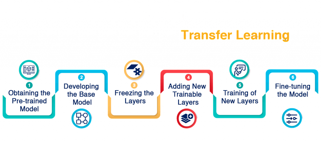
Two main approaches:

Feature extraction: Keep the pre-trained model fixed and train only the final classifier.

Fine-tuning: Retrain part of the network to adapt to the new domain.

Transfer learning embodies the same principle as Bayes’ Theorem — updating prior knowledge with new evidence to make better predictions.




Looking to Master Machine Learning? Discover the Machine Learning Expert Masters Program Training Course Available at ACTE Now!




Feature Engineering for Machine Learning

In any model, the quality of input features matters more than the choice of algorithm. Feature engineering involves transforming raw data into informative inputs.

Key steps include:

• Handling missing values (mean, median, or model-based imputation).
• Encoding categorical variables (one-hot, label, or ordinal encoding).
• Normalizing and scaling numerical data.
• Creating interaction or polynomial features.
• Selecting relevant features using techniques like mutual information or recursive feature elimination.

Tools such as Pandas, Scikit-learn, and Featuretools make this process systematic. High-quality features often allow even simple models like Naive Bayes to outperform more complex models with poor inputs.

Machine Learning Sample Resumes! Download & Edit, Get Noticed by Top Employers! Download

The F1 Score in Machine Learning

Evaluating models fairly is as important as building them. The F1 Score combines precision (how many predicted positives are correct) and recall (how many actual positives were identified) into a single metric:

• F1 = 2 \times \frac{Precision \times Recall}{Precision + Recall}

This metric is crucial in imbalanced datasets — for instance, in spam filtering or fraud detection, where the negative class dominates. It ensures that neither precision nor recall alone skews the evaluation.




Preparing for Machine Learning Job Interviews? Have a Look at Our Blog on Machine Learning Interview Questions and Answers To Ace Your Interview!




Conclusion

Understanding Naive Bayes and related foundational topics like HMMs, transfer learning, feature engineering, F1 score, recommendation systems, time series analysis, and the bias-variance tradeoff provides a panoramic view of machine learning’s landscape. Naive Bayes shows that elegant mathematics and sound probabilistic reasoning can achieve powerful, interpretable results even in today’s data-intensive world. As algorithms evolve, the principles of Bayes learning from evidence and updating beliefs remain at the core of intelligent systems machine learning training. From spam detection to medical diagnostics and beyond, the Naive Bayes theorem continues to illuminate how probability, data, and logic intertwine to turn uncertainty into understanding.