40+ [REAL-TIME] Pandas Interview Questions And Answers

Pandas is a robust Python library tailored for data manipulation and analysis. It provides flexible data structures like DataFrames and Series, enabling users to efficiently manage and analyze large datasets. With user-friendly functions for data cleaning, transformation, and visualization, Pandas is vital for data scientists and analysts seeking to extract insights from their data. Additionally, its seamless integration with other libraries such as NumPy and Matplotlib enhances its functionality for thorough data analysis.

1. What is pandas, and how does it differ from NumPy?

Ans:

The Panda’s library is a native Python library for data analysis. It extends the data structures available in the ‘Series’ and ‘DataFrame’ objects so that data can have labels. NUMPY provides important functionality for numerical computing because most operations are multidimensional arrays for rapid computation. It centres around the efficient calculation of homogeneous data; pandas extend the functionality of numPy by including the ability to manipulate and analyze heterogeneous and structured data, especially missing values and labels.

2. How to convert a dictionary to a pandas DataFrame?

Ans:

Use ‘pd.DataFrame(dictionary)’; the dictionary keys become column names, and the values become the data for the column. The dictionary values can be lists or arrays. Such a transformation takes structured data in dictionaries and arrays and converts it into a structured format, a DataFrame, which is highly useful for exploration and analysis. This allows users to leverage powerful pandas functionalities for data manipulation, filtering, and visualization, making it easier to derive insights from the data.

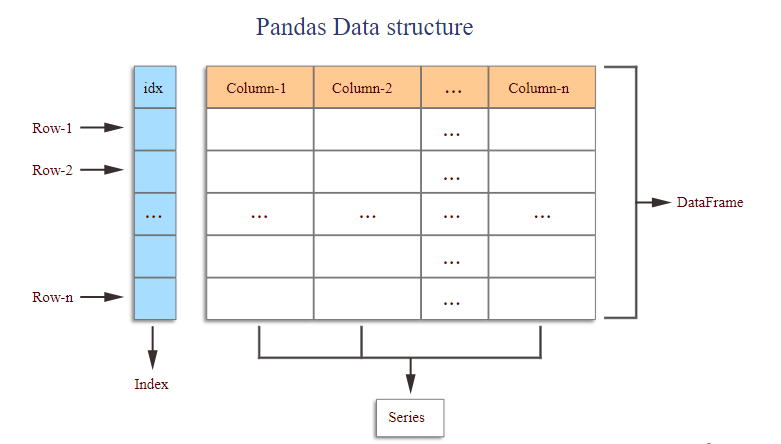
3. What about ‘Series’ and ‘DataFrame’ in pandas?

Ans:

• This structure is called a ‘Series’. It can be considered a one-dimensional labelled array holding any data type. 
• A ‘DataFrame’ is a two-dimensional table with rows and columns, each representing a ‘Series’. 
• ‘DataFrame’ is much more flexible, allowing multidimensional data manipulation.

4. How can a pandas DataFrame be converted into a NumPy array?

Ans:

• A pandas DataFrame can be transformed into a NumPy array with either the ‘df.to_numpy()’ method or the ‘df. Values’ attribute. 
• The former effectively strips away all DataFrame labels and returns only raw data in array form. One such array is very suitable for numerical computation, as it is free of any labels associated with the DataFrame. 
• It is possible to apply the NumPy functions and operations directly on it, and it improves performance when working solely with numeric data in most analytical tasks.

5. How to handle missing data in pandas?

Ans:

Pandas provides several methods to handle missing data efficiently, such as the ‘isna()’, ‘fill ()’, and ‘drop ()’ functions. The ‘isna()’ function determines missing values and returns a boolean DataFrame. To replace missing values, use the ‘fill ()’ method to pass replacement values. Otherwise, the ‘drop ()’ function removes rows or columns containing missing values. These methods are important in cleaning up and preparing data with accuracy and integrity.

6. Can rows or columns with missing values be deleted?

Ans:

Remove rows containing missing values, and use the ‘df. dropna(axis=0)’ command. It filters out the entire row with missing entries to clean the data set. For columns, the same operation is performed by the command ‘df. Drop a (axis=1)’, in which case any column containing missing entries will be removed. This helps delete the irrelevant data points in the data set so that an error-free data set is obtained. However, special caution must be exercised that some useful data is not deleted in error.

7. How can missing values be filled in a pandas data frame? 

Ans:

• One fills missing values in a data frame using ‘df. fillna(value)’. The ‘value’ here may be an explicit numeric value, the forward-fill method like ”fill”, or even values derived from other columns. 
• This preserves the data frame’s structure while filling gaps created by missing values. It prevents analysts from losing precious rows and maintains data continuity. 
• It is an important methodology in preprocessing datasets before further analysis and modelling.

8. How can columns of a data frame be renamed?

Ans:

• Rename columns of a DataFrame by passing a dictionary to the ‘df.rename(columns={‘old_name’: ‘new_name’})’. The keys are the original column names, and the values are the new names. 
• Such renaming makes the dataset much easier to read and, thus, understand. It could also conform column names to standards for certain naming conventions that an analysis might demand. 
• This flexibility enhances the organization and usability of data for various analytical tasks.

9. What is the difference between ‘.loc[]’ and ‘.iloc[]’ in pandas?

Ans:

Feature	‘.loc[]’	‘.iloc[]’
Indexing Method	Label-based indexing	Position-based indexing
Access Type	Accesses rows and columns using labels	Accesses rows and columns using integer indices
Syntax	‘df.loc[row_label, column_label]’	‘df.iloc[row_index, column_index]’
Includes Endpoints	Includes the endpoint in slicing	Excludes the endpoint in slicing
Suitable for	Accessing data based on specific labels	Accessing data based on integer positions

10. How can a CSV file be read into a pandas frame? 

Ans:

Import data from a CSV file into a pandas DataFrame using the command ‘pd.read_csv(‘file. csv’)’. The function reads the data automatically, making inferences about column names and data types for convenience. Importing from CSV files is easy and can enable a direct journey from raw data to structured analysis. As a result, pandas are ideal for data manipulation and analysis work. After loading the data, further study and processing can be done smoothly.

11. Which command selects a column from a pandas DataFrame?

Ans:

• A DataFrame column can be accessed using ‘df[‘column_name’]’ or ‘df.column_name’. This will return a pandas ‘Series’, a one-dimensional array for the values in the column. 
• If the column name has spaces or contains special characters, it only supports bracket notation ‘df[‘column_name’]’. 
• This way of access is convenient when you want to access just one column. A list of column names must be supplied to access more than one column.

12. How can missing data be identified in a pandas data frame?

Ans:

To find missing data inside a DataFrame, the functions ‘df. isna()’ or ‘df. isnull()’ can be called very efficiently. These functions will return a DataFrame full of boolean values, where ‘True’ points to missing entries while ‘False’ refers to present ones. It is immediately visual; thereby easy for the quick assessment of the quality of the data. To summarise missing values, one can use the command ‘df. ISNA ().sum()’ to count the missing entries in all columns. This information is crucial to identify which missing data to address in the subsequent analyses.

13. How to index a row by position in pandas?

Ans:

• Rows can be accessed by their position with ‘.iloc[]’. For instance, ‘df.iloc[0]’ returns the first row, and ‘df.iloc[2:5]’ returns rows 3 to 5. 
• This position-based access method doesn’t care about the rows’ actual labels; it only depends on their numeric location in the data frame. 
• This is useful for extracting rows when the positions are known. For more advanced selections, it can also be accessed with slicing and lists of indices.

14. How would one filter rows from a pandas DataFrame, say, based on the values of columns?

Ans:

Apply boolean condition for filtering rows on column values. For example, ‘df[df[‘column_name’] > value]’ returns the rows where the column values are more than that of the given value. It produces a boolean mask that filters the DataFrame. Multiple conditions can be used to create very complex filters. It is very flexible in data exploration and manipulation.

15. How to select multiple columns in pandas?

Ans:

Passing a list of column names allows multiple columns to be selected. For example, ‘df[[‘col1’, ‘col2′]]’ returns a DataFrame with only those columns of interest. The column names must, however, be passed within double brackets, as this is the syntax for differentiating between a list of columns and selecting a single column. This facilitates choosing multiple features from a data set for closer investigation or analysis. Both labelled and positional column selections work.

16. How to set an index for a data frame?

Ans:

• To set an index, use ‘df.set_index(‘column_name’)’ This assigns the values in the column passed as the new row labels.    
• The old integer index is replaced, and the data can now be accessed using the new index. This might be helpful when more meaningful identifiers, such as IDs or timestamps, already exist and are better described by the rows. 
• The method also offers choices whether should drop the original column or retain it. Indexing hastens the lookup of data.

17. How to reset the index of a data frame?

Ans:

• Use ‘df.reset_index()’ to return the index to a default integer index. This function drops the current index so that it reverts to its numeric default range. 
• The previous index can optionally be kept as a column using the parameter ‘drop=False’.
• Resetting the index is very useful when the previous one is no longer needed or after executing one or more operations that have altered the original indexing of the data. This helps organize the data for further analyses.

18. Filter rows with conditions on multiple columns in pandas.

Ans:

Boolean operators, ‘&’ for and, or ‘|’ for or, are essential for filtering data in pandas. For example, ‘df[(df[‘col1’] > value1) & (df[‘col2’] < value2)]’ will return the rows where both conditions are met; therefore, the conditions must be enclosed in parentheses, with ‘&’ or ‘|’ used between them. This method is particularly useful for achieving a more granular level of data selection. By combining multiple conditions, analysts can refine their queries to extract precisely the data they need for analysis.

19. What is multi-indexing, and how to generate it in pandas?

Ans:

Multi-indexing, or hierarchical indexing, enables a data frame to have multiple row or column label levels. It helps deal with any dataset with intricate structure, such as a time series with many identifiers. A MultiIndex can be created using ‘pd.MultiIndex.from_arrays()’ or setting multiple columns as an index using ‘set_index()’. Multi-indexing aids in more elaborate analysis and slicing on various dimensions. This improves the structures for organizing and retrieving complex data.

20. How to extract unique values in the Panda’s column?

Ans:

• Can get the list of unique values in a column using ‘df[‘column_name’].unique()’, which returns an array of all the unique entries in the given column. 
• This could be useful if you need to determine how many categories or unique rows exist in a dataset. To count unique values across a really large Series, use ‘pd.Series. unique ()’. 
• The ‘unique()’ function efficiently understands the data distribution, especially in categorical columns, because it simplifies finding repetitive or missing categories. 

21. How do you add a new column to pandas DataFrame?   

Ans:

• Add new columns by assigning their values, such as ‘df[‘new_column’] = values’.   
• The values can be any type: list, numpy array or any computation involving existing columns. If assigned a scalar, then the whole column will be filled with this scalar. 
• The default is to append columns to the right side of the DataFrame. This function introduces dynamic extensibility to the data frame’s structure.

22. How does the user drop a column from a data frame?

Ans:

Dropping a column can be done using ‘df. drop(‘column_name’, axis=1)’. Here, ‘axis=1’ is used to indicate that a column is going to be dropped. This operation can be performed in-place by setting ‘inplace=True’ or it returns a new DataFrame without the column specified above. Multiple columns are removed simultaneously by passing a list of column names. It helps keep the DataFrame free from unwanted data.

23. How to sort the columns of pandas DataFrame?

Ans:

A column can be reordered using the names of columns inside list brackets in the order in which one wants these, for example: ‘df = df[[‘col3’, ‘col1’, ‘col2′]]’. This command creates a new DataFrame with columns reordered as specified. It is straightforward to adjust column positions according to needs in an analysis. Reordering draws attention precisely to certain data or makes it more readable inside the DataFrame.

24. How to apply a function to each element in a pandas column?

Ans:

• The function can be applied to every element of the Panda’s column using the method ‘.apply()’, which is something like this: ‘df[‘column_name’].apply(function)’. 
• This applies a given function to each element to process it and returns one new Series containing all the results of the function application. 
• It is handy to perform element-wise operations or transformations, like formatting or calculations. Of course, this is also a good way to make the data manipulation in a data frame more flexible.

25. What does ‘apply()’ with a lambda function do in pandas?

Ans:

• .apply() to be combined with lambda functions to perform every element-related operation, as in df[‘column_name’].apply(lambda x: x + 1). 
• Thus, applying a lambda function returns every value in the column under consideration to transform them elegantly. 
• It enables direct customization modifications without defining a separate function for quick changes. It is economical for simple operations directly in a DataFrame context.

26. How to sort a pandas data frame on one column?

Ans:

There is ‘.sort_values(‘column_name’)’ to sort a pandas DataFrame on one column. By default, it returns the DataFrame for ascending order, though ‘ascending=False’ may be specified to get a reverse sort. Sorting data helps sort data based on given attributes so that it can easily be analyzed or plotted. The ‘sort_values()’ method returns a new object and leaves the original object unchanged unless specified with the ‘inplace=True’ parameter.

27. How to sort a data frame with multiple columns?

Ans:

With the ‘.sort_values()’ method, multiple columns in a DataFrame can be sorted by passing through a list of column names, like ‘df.sort_values([‘col1’, ‘col2′])’. The values will be sorted first by ‘col1’ and then by ‘col2’ for tied values. The ‘ascending’ parameter accepts a list defining sorting order for each column. The method can perform complex data organization based on many data attributes. This improves the precision of data analysis.

28. How to group the data using pandas?

Ans:

• Data can be grouped using the method ‘.groupby()’, for example, ‘df. group by (‘column_name’)’. The data frame is separated into groups depending on the unique values in that column. 
• It allows aggregated calculations on those groups. Aggregation functions like sum(), mean() or count() can be applied afterwards to calculate statistics. 
• Grouping is good for aggregating data and performing for aggregating data and performing operations on the DataFrame subsets.

29. How to calculate aggregate statistics using pandas? 

Ans:

• There are aggregate statistics that can be computed after grouping by using the ‘.agg()’ method, for example: ‘df.groupby(‘column_name’).agg({‘other_col’: ‘mean’})’. 
• This calculates the mean of ‘other_col’ by groups of unique values in ‘column_name’. A dictionary format can be used to compute multiple aggregate functions at once. 
• This function simplifies data analysis by returning a set of summary statistics for all categories or groups in a data frame.

30. How to find duplicate rows in pandas DataFrame?

Ans:

Duplicates may be checked with ‘df. duplicated()’ returns a boolean Series indicating if a row is a duplicate of some previous row. To get which rows are duplicates, use ‘df[df.duplicated()]’. The ‘keep’ parameter determines which of the duplicates shall be marked-all of them (‘False’), the first one (‘first’), or the last one (‘last’). This helps in cleaning up data by detecting and handling repeated entries.

31. How can two Pandas DataFrames be concatenated?

Ans:

It is possible to concatenate two pandas DataFrames using the ‘pd. concat([df1, df2])’ function. The latter stacks vertically or horizontally according to the axis specified. The default setting is to concatenate along rows, ‘axis=0’. You can set the ‘ignore_index’ parameter to ‘True’ to reset the index in the resulting DataFrame. That method can combine multiple data frames very efficiently for comprehensive analysis.

32. What is the difference between ‘merge()’ and ‘join()’ in pandas?

Ans:

• Merge() is used to merge DataFrames based on common columns or indices, similar to SQL joins.
• It allows for more complex merge operations, including inner, outer, left, and right joins. The ‘join()’ function is more simplistic and mainly intended for index-joining. 
• They both combine data frames, but the use case is different.

33. How to merge DataFrames on specific columns?

Ans:

• The ‘PD.merge(df1, df2, on=’column_name’)’ function can merge DataFrames on specified columns. It merges ‘df1’ and ‘df2’ according to the column name in the argument.
• Another argument, ‘how’, determines the type of merge: ‘inner’, ‘outer’, ‘left’, or ‘right’. This provides flexibility for merging datasets for analysis. Overall, this functionality is essential for combining related data effectively.

34. How do users perform an inner join on pandas?

Ans:

Users can use the ‘PD. merge (df1, df2, how=’inner ‘, on=’column_name ‘)’ to perform an inner join. This technique merges rows from both data frames with matches in this column. It excludes rows without a match in the result’s first or second data frame. Inner joins are useful in retaining only the common entries between two datasets for further analysis so that only relevant data is analyzed.

35. How do users do an outer join in pandas?

Ans:

Users can do an outer join using ‘pd. merge (df1, df2, how=’outer ‘, on=’column_name ‘) ‘. This function merges both DataFrames by bringing all rows from either the left or the right DataFrame and filling in NaN where there are no matches. In the case of outer joins, all entries are captured, whether or not a match exists in both data. Outer joins are useful for detailed data analyses, where every information can be considered and the gaps and mismatches between them identified.

36. How to perform a left join in pandas?

Ans:

A left join is called ‘pd. merge(df1, df2, how=’left’, on=’column_name’)’. This method leaves all the rows of the left DataFrame (‘df1’) and merges the entries from the right DataFrame (‘df2’). NaN values fill in for any without a match. Left joins can then be utilized to keep one dataset from one data frame while bringing in matching data from another.

37. How to do a right join in pandas?

Ans:

• A right join can be performed with ‘pd.merge(df1, df2, how=’right’, on=’column_name’)’. 
• This maintains all rows from the right DataFrame, ‘df2’ while matching entries with the left one, ‘df1’. The final result will fill the remaining unmatched rows in ‘df1’ with NaNs. 
• Right joins are applicable when all data from one DataFrame needs to be included but supplemented by appropriate entries from another.

38. How to join DataFrames on the index?

Ans:

• The function ‘pd. Merge (df1, df2, left_index=True, right_index=True)’ allows you to join DataFrames by their indices. 
• This method aligns rows based on their index values instead of specific columns. Merging DataFrames where the index represents meaningful relations is convenient. 
• Index-merging simplifies the operations when column names do not match or are not provided.

39. What does ‘concat()’ mean in pandas?

Ans:

The ‘Concat ()’ function in pandas unites multiple DataFrames along any specified axis, either vertically or horizontally. The following methods invoke this function: It is used for vertical concatenation as follows: ‘pd.concat([df1, df2], axis=0) and for horizontal concatenation as follows:axis=1’. The flexibility of this function combines data from various sources and can merge them either by keeping the indices or resetting them. It is widely used to aggregate data in batch operations or from different sources.

40. How to concatenate one DataFrame with another in pandas?

Ans:

Another common method for appending one data frame to another is the ‘df1.append(df2)’ method, which stacks ‘df2’ below ‘df1’. This leaves the index from ‘df1’ and adds ‘df2’ as new rows. Using the ‘ignore_index’ parameter with ‘True’ will create a new integer index in the resulting DataFrame; an example is as follows: If data can be augmented with extra entries, appending is a particularly efficient way to combine them.

41. How to create a pandas DataFrame with date information?

Ans:

A pandas data frame can be initialized with date information by including a column of dates. For example, ‘pd.DataFrame({‘dates’: pd.to_datetime([‘2023-01-01’, ‘2023-02-01′])})’ creates a DataFrame containing a date column. The ‘pd.date_range()’ function can generate a sequence of dates. This feature is beneficial for conducting time series analysis and allows for manipulating date-related data directly within the data frame.

42. How to convert a column to datetime format?

Ans:

• A column can be converted to datetime format using the ‘pd.to_datetime()’ function. For instance, executing ‘df[‘date_column’] = pd.to_datetime(df[‘date_column’])’ changes the specified column into datetime objects. 
• This conversion is crucial for executing time-based operations and analyses. The function can recognize various date formats automatically. 
• Proper datetime formatting ensures accurate calculations and filtering based on dates.

43. How can the year, month, or day be extracted from a datetime column?

Ans:

The year, month, or day from a datetime column can be extracted using the ‘.dt’ accessor. For example, ‘df[‘year’] = df[‘date_column’].dt.year’ retrieves the year, while ‘df[‘month’] = df[‘date_column’].dt.month’ and ‘df[‘day’] = df[‘date_column’].dt.day’ allows for the extraction of the month and day, respectively. This functionality is essential for conducting a detailed analysis of date components, enabling further data manipulation and aggregation based on specific time elements.

44. How to filter data between two dates in pandas?  

Ans:

Filtering data between two dates can be done through boolean indexing, such as ‘df[(df[‘date_column’] >= ‘2023-01-01’) & (df[‘date_column’] <= ‘2023-12-31′)]’. This expression returns rows where the date falls within the defined range. The comparison operators facilitate flexible date filtering, ensuring only relevant entries are included. This method is vital for analyzing time-bound data within a specified period.

45. What is resampling in time series, and how to use it in pandas?  

Ans:

• Resampling in time series refers to altering the frequency of time series data, allowing for aggregation or interpolation over designated intervals. 
• This can be accomplished using the ‘.resample()’ method, such as ‘df.resample(‘M’).mean()’ to compute monthly averages. 
• Resampling enables time series data analysis at various granularities, allowing for insights over different periods. It is particularly useful for summarizing and visualizing trends.

46. How to perform forward and backward filling in time series?

Ans:

• Forward and backward filling can be executed using the ‘.fillna()’ method in pandas. 
• Forward filling replaces NaN values with the last non-null value through ‘df. fill (method=’ffill’)’, while backwards filling fills NaNs with the subsequent known value using ‘df. fillna(method=’bfill’)’. 
• These techniques are instrumental in maintaining continuity in time series data by effectively addressing missing values. Filling methods enhance data completeness for accurate analysis.

47. How to calculate the rolling average of a column?  

Ans:

The rolling average can be calculated using the ‘.rolling(window).mean()’ method. For example, ‘df[‘rolling_avg’] = df[‘column_name’].rolling(window=3).mean()’ computes the average over a specified window size of 3. This operation generates a new Series containing the rolling average, facilitating the smoothing of time series data. Rolling averages effectively identify trends and patterns by reducing noise in the data.

48. How to shift data in time series using pandas?  

Ans:

Data shifting in a time series can be achieved through the ‘.shift()’ method, such as ‘df[‘shifted’] = df[‘column_name’].shift(1)’. This method shifts the data by a specified number of periods, introducing NaNs in the shifted positions. Shifting is useful for comparing current data with past values, allowing for calculations involving changes or lagged variables. It enhances time series analysis by enabling the examination of previous observations.

49. How to handle time zone-aware data in pandas? 

Ans:

• Time zone-aware data can be managed by assigning time zones using the ‘.dt.tz_localize()’ method, such as ‘df[‘date_column’] = df[‘date_column’].dt.tz_localize(‘UTC’)’. 
• Conversions between time zones can be performed using ‘.dt.tz_convert(‘America/New_York’)’. This functionality ensures accurate handling of datetime objects across different time zones. 
• Time zone awareness is essential for synchronizing data from various geographical locations.

50. How to compare time series data across different time zones in pandas?  

Ans:

• Time series data across different time zones can be compared by standardizing to a common time zone using the ‘.dt.tz_convert()’ method. 
• For example, converting all dates to UTC ensures consistent comparisons. Once aligned, standard operations like merging or plotting can be performed effectively. 
• This approach guarantees that discrepancies caused by time zone differences do not impact the analysis or interpretation of the data.

51. How to pivot a pandas DataFrame? 

Ans:

A data frame can be pivoted using the ‘.pivot()’ method, such as ‘df. pivot(index=’index_column’, columns=’column_to_pivot’, values=’values_column’)’. This operation restructures the DataFrame by converting unique values from one column into new columns, with the index specified. Pivoting is beneficial for organizing data into a more interpretable format, particularly for summarizing values based on categories. It simplifies the analysis of multidimensional data.

52. What is the difference between ‘melt()’ and ‘pivot()’ in pandas? 

Ans:

The ‘melt()’ function transforms a data frame from wide to long format, collapsing multiple columns into key-value pairs. Conversely, ‘pivot()’ reshapes data from long to wide format, generating new columns from unique values in a designated column. While ‘melt()’ is designed for unpivoting data, ‘pivot()’ focuses on restructuring it. Both methods are essential for data manipulation, depending on the required format for analysis.

53. How to unstack a multi-index data frame? 

Ans:

• A multi-index data frame, such as df, can be unstacked using the ‘.unstack()’ method. unstack()’. 
• This method pivots the innermost index level into columns, producing a wider data frame. Unstacking is valuable for visualizing hierarchical data in a more user-friendly format. 
• It facilitates easier analysis and manipulation of multi-level indexed data, leading to better insights.

54. How to create a crosstab in pandas? 

Ans:

• A crosstab can be generated using the ‘pd.crosstab()’ function, such as ‘pd.crosstab(df[‘column1’], df[‘column2′])’. 
• This function computes a simple cross-tabulation of two or more factors, resulting in a data frame that displays occurrence counts. 
• Crosstabs are useful for analyzing the relationships between categorical variables, providing a clear view of their interactions. This method enhances the exploration of categorical data distributions.

55. What is a pivot table in pandas, and how to create one?  

Ans:

A pivot table is a data summarization tool for aggregating data based on specific variables. It can be created using the ‘pd.pivot_table()’ function, such as ‘pd.pivot_table(df, values=’values_column’, index=’index_column’, columns=’column_to_pivot’, aggfunc=’mean’)’. This function allows for flexible aggregations, such as sum, mean, or count, and rearranges the data for easier analysis. Pivot tables are crucial for efficiently summarizing complex datasets.

56. How to rank values in a pandas DataFrame?

Ans:

Values can be ranked using the ‘.rank () ‘method, such as ‘df [‘ranked ‘] = df [‘column_name ‘] .rank (). This method assigns a rank to each value in the specified column, with ties receiving the same rank by default. Different ranking methods, including average, min, or max, can be selected. The ranking is useful for ordinal analysis and comparisons among data points, enhancing the interpretation of results.

57. How to quantile-bin data in pandas?  

Ans:

• Data can be quantile-binned using the ‘pd.qcut()’ function, which divides the data into equal-sized bins based on quantiles. 
• For example, ‘df[‘binned’] = pd.qcut(df[‘column_name’], q=4)’ creates quartiles. This method assigns each value to a corresponding bin, aiding the categorical analysis of continuous data. 
• Quantile-binning assists in understanding data distribution and categorizing it for better insights.

58. How to calculate the cumulative sum of a column in pandas?  

Ans:

• The cumulative sum can be calculated using the ‘.cumsum()’ method, such as ‘df[‘cumsum’] = df[‘column_name’].cumsum()’. 
• This method generates a new series that displays the cumulative total at each index. Cumulative sums are useful for tracking progressive totals over time or across categories, offering insights into trends and patterns in the data. It enhances the analysis of sequential data.

59. How to handle categorical data in pandas? 

Ans:

Categorical data can be effectively managed using the ‘pd.Categorical()’ function, converting a column into a categorical type. This approach optimizes memory usage and improves performance for data analysis. Additionally, categorical data can be assigned an order, allowing for ordered comparisons. Proper handling of categorical data is essential for effective analysis, facilitating operations such as grouping and aggregation.

60. How to get a random sample of rows from a pandas DataFrame?  

Ans:

Using the ‘.sample()’ method, such as ‘df. sample(n=5)’ to retrieve 5 random rows, a random sample of rows can be obtained. This function allows specifying the number of samples or a fraction of the total data frame. Random sampling is beneficial for creating representative subsets for analysis or validation, ensuring that the selected sample accurately reflects the larger dataset. This method enhances the robustness of data-driven conclusions.

61. How to optimize pandas’ operations for performance? 

Ans:

• Performance optimization in pandas can be achieved by minimizing loops, leveraging vectorized operations, and applying built-in functions. 
• It is recommended that you use ‘apply()’ judiciously, as it can be slower than native operations. Additionally, utilizing ‘categorical’ data types helps reduce memory consumption. 
• Employing the ‘numba’ library for JIT compilation can further enhance performance for computationally intensive operations. 
• Lastly, profiling code with tools like ‘line_profiler’ can help identify bottlenecks for targeted optimization.

62. What is the purpose of using ‘categorical’ data types in pandas?  

Ans:

• The ‘categorical’ data type in pandas is utilized to optimize memory usage and improve performance, particularly with large datasets containing repeated values. 
• By converting string columns to categorical types, storage requirements are significantly reduced, as categories are stored as integer codes. 
• Categorical types also facilitate faster comparisons and enable better data processing capabilities. Furthermore, they allow for ordered categories, enhancing the functionality for certain analytical tasks and visualizations.

63. How to reduce the memory usage of a pandas DataFrame?

Ans:

Memory usage of a pandas DataFrame can be reduced by changing data types to more efficient formats, such as converting ‘float64’ to ‘float32’ or ‘int64’ to ‘int32’. Employing ‘categorical’ types for columns with repetitive string values can also help. Additionally, dropping unnecessary columns or rows can minimize memory consumption. Using the ‘df.memory_usage(deep=True)’ method provides insight into memory allocation for optimization. Employing chunking when loading large datasets helps manage memory more effectively.

64. How to load large CSV files in chunks using pandas? 

Ans:

Large CSV files can be loaded in chunks using the ‘pd.read_csv()’ function with the ‘chunksize’ parameter. For example, ‘for chunk in pd.read_csv(‘file. csv’, chunksize=1000):’ processes the file in segments of 1000 rows. This approach allows for manageable memory consumption and facilitates processing datasets too large to fit in memory. Each chunk can be analyzed individually, and results can be aggregated later. This method is particularly useful for data cleaning and transformation tasks.

65. How to parallelize operations in pandas?  

Ans:

• Operation parallelization in pandas can be achieved by using libraries such as Dask or Modin. Dask allows for out-of-core computations and can parallelize pandas operations across multiple CPU cores, enabling the processing of larger-than-memory datasets. 
• Modin offers a drop-in replacement for pandas, automatically leveraging parallelization. Utilizing Python’s ‘multiprocessing’ module can also enhance performance for operations that can be divided into smaller tasks. 
• This improves computational efficiency for large data processing tasks.

66. How do pandas handle large datasets that don’t fit into memory?

Ans:

• Pandas can handle large datasets that exceed memory limits through various techniques, such as using Dask or loading data in chunks with the ‘pd.read_csv()’ method. 
• Dask provides a parallelized environment for out-of-core processing, allowing operations on large datasets as if they were in memory. 
• Additionally, filtering and preprocessing data during loading can reduce memory footprint. 
• Leveraging data formats like HDF5 or Parquet enables efficient reading and writing of large datasets while minimizing memory usage.

67. What is Dask, and how does it integrate with pandas?  

Ans:

Dask is a flexible parallel computing library for Python that integrates seamlessly with pandas to enable large-scale data processing. It provides a DataFrame structure similar to pandas, allowing operations to be performed in parallel across multiple cores or distributed systems. Dask’s lazy evaluation model optimizes resource utilization, executing tasks only when necessary. This integration allows for efficient handling of datasets that don’t fit into memory, enabling scalable data analysis and manipulation while maintaining pandas-like syntax.

68. How to optimize merge operations in pandas for large data?  

Ans:

To optimize merge operations in pandas for large datasets, it is essential to ensure that merging columns are of the same data type, as mismatched types can slow down the operation. Using indexes can also speed up merges; setting an index on the merging columns via ‘set_index()’ is recommended. Utilizing the ‘how’ parameter to specify the type of join (e.g., inner, outer) effectively reduces the size of the resulting data frame. Additionally, filtering out unnecessary columns before merging helps minimize data load.

69. How to profile pandas operations to identify performance bottlenecks?

Ans:

• To analyze runtime and memory usage, profiling pandas operations can be accomplished using libraries such as ‘line_profiler’ or ‘memory_profiler’. 
• Using the ‘% time’s magic function in Jupyter Notebooks helps assess the execution time of specific code blocks. The ‘pandas_profiling’ library also comprehensively reports DataFrame characteristics and potential issues. 
• These tools help identify bottlenecks in code, guiding targeted optimization efforts for improved performance in data processing tasks.

70. What is the benefit of using ‘pd.eval()’ in pandas? 

Ans:

• The ‘PD.eval()’ function allows for the more efficient evaluation of expressions, leveraging NumPy’s capabilities for faster computations. 
• It supports operations such as filtering, arithmetic, and assigning new columns in a more concise syntax. Using ‘pd. eval()’ can reduce the overhead of intermediate variables, leading to improved performance, especially with large DataFrames. 
• This method is particularly useful for complex calculations, offering a cleaner and faster way to perform operations on Panda objects.

71. How to plot a pandas DataFrame? 

Ans:

A pandas data frame can be plotted using the ‘.plot()’ method, providing a high-level interface for creating various visualizations. For example, calling ‘df. Plot ()’ generates a line plot by default. This method integrates seamlessly with Matplotlib, allowing customized plot attributes such as titles, labels, and styles. Additional plot types can be specified using the ‘kind’ parameter, such as ‘df. Plot (kind=’bar’)’ for bar plots. This flexibility makes it easy to visualize data insights.

72. How to create a line plot using pandas? 

Ans:

A line plot can be created using the ‘.plot()’ method on a DataFrame or Series. For instance, executing ‘df[‘column_name’].plot()’ generates a line plot of the specified column. Customization options allow for modifications like labels and titles, such as ‘df[‘column_name’].plot(title=’My Line Plot’, ylabel=’Values’)’. This method leverages Matplotlib for additional styling capabilities. Line plots are particularly effective for visualizing trends over time or continuous data.

73. How to create a bar plot using pandas?  

Ans:

• A bar plot can be generated using the ‘.plot()’ method by specifying the ‘kind’ parameter as ‘bar’. 
• For example, ‘df[‘column_name’].value_counts().plot(‘)’kind=’ bar creates a bar chart showing the frequency of values in a column. This visualization is effective for comparing categorical data. 
• Customization options, such as setting titles and adjusting colours, enhance the presentation. Bar plots provide a clear and concise way to visualize relationships among categorical variables.

74. How to create a scatter plot using pandas?  

Ans:

• A scatter plot can be created using the ‘.plot.scatter()’ method or the general ‘.plot()’ method with ‘kind=’scatter”. 
• For instance, ‘df.plot.scatter(x=’x_column’, y=’y_column’)’ generates a scatter plot of the specified columns. This visualization effectively illustrates relationships and correlations between two numerical variables. 
• Customizations such as colour mapping and marker styles can enhance the plot’s clarity. Scatter plots are particularly useful for detecting patterns and outliers in data.

75. How to plot a histogram using pandas?

Ans:

A histogram can be plotted using the ‘.hist()’ method or the ‘.plot.hist()’ method on a data frame or Series. For example, ‘df[‘column_name’].hist(bins=30)’ creates a histogram with 30 bins. This visualization helps to understand the distribution of a continuous variable, providing insights into frequency counts across ranges. Customization options such as colour and edge width enhance the appearance of the histogram. Histograms are effective for analyzing the distribution and spread of data.

76. How to create subplots in pandas?  

Ans:

Subplots can be created using the ‘plt.subplots()’ function from Matplotlib in conjunction with pandas plotting capabilities. For example, ‘fig, axs = plt.subplots(nrows=2, ncols=2)’ sets up a 2×2 grid for subplots. Individual DataFrame columns can be plotted in each subplot by passing the appropriate axes object. Customizations for each subplot can be applied independently, allowing for tailored visualizations. This method provides a cohesive way to present multiple related plots in one figure.

77. How to visualize time series data using pandas?

Ans:

• Time series data can be visualized using the ‘.plot()’ method, which automatically formats the x-axis as dates if the index is DateTime. For instance, ‘df.plot()’ effectively visualizes trends over time. 
• Additional options, such as specifying ‘kind=’line,’ enhance clarity. Matplotlib, with its grid lines and annotations, can be utilized for further customization, enriching the visualization. 
• This approach facilitates in-depth analysis of temporal trends and patterns.

78. How to customize the appearance of a plot created using pandas?  

Ans:

• The appearance of a pandas plot can be customized by modifying parameters within the ‘.plot()’ method, such as ‘title’, ‘xlabel’, and ‘ylabel’. 
• Furthermore, Matplotlib functions can be utilized for additional stylings, such as adjusting colours and line styles. For example, ‘df[‘column_name’].plot(‘color=’ red, linestyle=’–‘)’ alters the color and line style. 
• Saving plots in different formats using ‘plt.savefig()’ also contributes to presentation quality. Customizations enhance the readability and effectiveness of visualizations.

79. How to integrate pandas with libraries like Matplotlib or Seaborn?  

Ans:

Pandas integrates seamlessly with Matplotlib and Seaborn, leveraging their functionalities for enhanced data visualization. Using ‘import matplotlib. pyplot as plt’ or ‘import seaborn as sns’, plots can be generated directly from pandas DataFrames. For instance, ‘df. plot()’ utilizes Matplotlib, while ‘sns.scatterplot(data=df, x=’x_column’, y=’y_column’)’ employs Seaborn for improved aesthetics. Customizations from these libraries enhance the visual output, making it easier to communicate insights effectively.

80. How to save a plot created with pandas as an image file?

Ans:

A plot created with pandas can be saved as an image file using Matplotlib’s ‘saving ()’ function. After generating the plot, call ‘plot. savefig(‘plot. png’)’ saves the current figure in the specified format, such as PNG or PDF. Custom parameters include ‘dpi’ for resolution and ‘bbox_inches=’tight” for layout adjustment. This feature allows for easy sharing and documentation of visualizations. Saving plots ensures that insights can be preserved and presented effectively.

81. How to read data from a SQL database into a pandas DataFrame?  

Ans:

• Data can be imported from a SQL database into a pandas DataFrame using the ‘pd.read_sql_query()’ or ‘pd.read_sql_table()’ functions. 
• Establishing a connection to the database typically involves libraries like SQLAlchemy or SQLite3. For instance, executing ‘df = pd.read_sql_query(‘SELECT * FROM table_name’, connection)’ pulls data from the specified table. 
• This method facilitates the smooth integration of SQL data into pandas for further analysis and processing. Proper database connection management is essential for effective data retrieval.

82. How to write data from a pandas DataFrame to a SQL database?

Ans:

• Data from a pandas DataFrame can be exported to a SQL database using the ‘to_sql()’ method. 
• This function defines the target table and connection details, such as ‘df.to_sql(‘table_name’, connection, if_exists=’replace’)’, which replaces the table if it exists. 
• The ‘index’ parameter can be set to ‘False’ to prevent the DataFrame index from being written as a column. This feature enables efficient data storage and updating in SQL databases directly from pandas, streamlining data management.

83. How to execute SQL queries using pandas?

Ans:

SQL queries can be run using pandas by utilizing the ‘pd.read_sql_query()’ function, which supports direct execution of SQL statements. By providing a SQL query string along with a database connection, such as ‘df = pd.read_sql_query(‘SELECT * FROM table_name WHERE condition’, connection)’, the results are returned as a DataFrame. This capability allows for using complex SQL queries for data extraction and manipulation, integrating SQL’s power with pandas for data analysis.

84. How to perform complex SQL-like joins in pandas? 

Ans:

Complex SQL-like joins can be executed in pandas using the ‘merge()’ function, which supports various join types, including inner, outer, left, and right joins. For example, ‘pd.merge(df1, df2, on=’key’, how=’inner’)’ combines two DataFrames based on a shared key. The ‘indicator’ parameter can be used to identify the source of each row, similar to SQL’s JOIN operations. This functionality allows for flexible data integration, effectively mimicking SQL joins within pandas.

85. How to handle missing or null values from a SQL query in pandas?

Ans:

• Missing or null values from a SQL query can be managed in pandas using methods such as ‘fillna()’ or ‘dropna()’. After retrieving data with null values, these methods facilitate imputation or removal. 
• For instance, ‘df. Fill (0)’ replaces missing values with zero, while ‘df. Drop a ()’ eliminates rows with null entries. 
• Additionally, handling NULLs can be addressed at the SQL query level using ‘COALESCE()’ or ‘IS NULL’ conditions to maintain data integrity before importing it into pandas.

86. How to load data from multiple database tables into a pandas DataFrame?

Ans:

• Data from multiple database tables can be loaded into Pandas DataFrame by executing various SQL queries or JOIN statements in a single query. 
• With ‘pd.read_sql_query()’, data can be fetched from a query that combines data across tables, such as ‘df = pd.read_sql_query(‘SELECT * FROM table1 JOIN table2 ON table1.id = table2.id’, connection)’. 
• This method allows for comprehensive data retrieval and analysis, consolidating related information from various sources into a single data frame.

87. How to work with NoSQL databases in pandas?

Ans:

• Interaction with NoSQL databases in pandas often involves using libraries such as PyMongo for MongoDB. Data can be retrieved using MongoDB queries and converted into a pandas DataFrame. 
• For example, after establishing a connection with ‘client = MongoClient()’, executing ‘data = pd.DataFrame(list(collection.find()))’ transforms queried documents into a DataFrame. 
• This integration facilitates analyzing and manipulating unstructured data typically stored in NoSQL databases.

88. What are the common methods for handling SQL databases in pandas? 

Ans:

Common methods for working with SQL databases in pandas include ‘pd.read_sql_query()’, ‘pd.read_sql_table()’, and ‘DataFrame.to_sql()’. These methods enable seamless interaction with SQL databases, facilitating data retrieval, execution of SQL commands, and data storage. Creating database connections using SQLAlchemy or SQLite3 is crucial for these operations. Additionally, pandas can execute complex SQL queries and perform data manipulations, effectively bridging SQL capabilities with DataFrame functionalities.

89. How to compare the performance of pandas vs SQL for large datasets?  

Ans:

Evaluating the performance of pandas versus SQL for large datasets involves assessing execution time and resource consumption for specific tasks. Benchmarking can be conducted by measuring the time required for data retrieval, aggregation, and transformations using pandas and SQL. Indexing, query optimization, and data storage formats can affect performance outcomes. Generally, SQL might perform better in large-scale data filtering and aggregation, while pandas excel in flexibility and in-memory manipulation.

90. How to use pandas with cloud databases like Amazon RDS or Redshift?

Ans:

To use pandas with cloud databases such as Amazon RDS or Redshift, establish a connection via SQLAlchemy or similar libraries. For example, ‘engine = create_engine(‘postgresql+psycopg2://user:password@host: port/name)’ enables connectivity to the database. Data retrieval can be done using ‘pd.read_sql_query()’ and data can be written back using ‘to_sql()’. This integration allows for scalable data analysis and manipulation in cloud environments, leveraging pandas’ powerful data processing capabilities on large datasets stored in cloud databases.