What is [MS] Excel & Tutorial? Defined, Explained, & Explored

Last updated on 19th Jul 2020, Blog, Tutorials

• When you open an Excel worksheet, you are presented with the Excel window. You use this window to interact with the software—you type your data into the window and you use the window to tell Excel what to do. In this section, I will explain the parts of the Excel window.

• A Quick Access Toolbar: In the upper-left corner of the window is the Quick Access toolbar, sometimes referred to as the QAT. The Quick Access Toolbar provides commands you frequently use. Save, Undo, and Redo appear on the toolbar by default. Click Save to save your file, Undo to roll back an action you have taken, and Redo to reapply an action you have rolled back.

• B Title Bar: In the top center of the window to the right of the Quick Access toolbar is the Title bar. The Title Bar displays the title of your workbook. Excel names the first new workbook you open Book1. As you open additional new workbooks, Excel names them sequentially. When you save a workbook, you assign the workbook a new name.

• C Help Button : The Help button, along with several other buttons, is located in the upper-right corner of the window. It takes you to the Excel help area. In the help area, you can search for information on how to perform tasks.

• D Ribbon Display Options Button : The Ribbon Display Options button is located next to the Help button. Use it to display the following menu options: Auto-hide Ribbon, Show Tabs, and Show Tabs and Commands. To learn more about these options, see the section The Excel Ribbon.

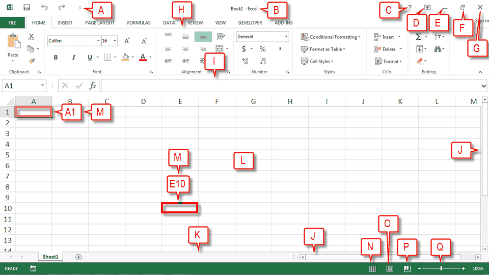
E Minimize Button : The Minimize button is located next to the Ribbon Display Options button. To remove Excel from view and place the Excel icon on the Windows taskbar, click the Minimize button. To restore Excel, click the Excel icon on the Windows taskbar.F Restore Down : The Restore Down button is located next to the Minimize button. The Restore Down button reduces the size of the Excel window. When you click the Restore Down button, it turns into the Maximize button.

Maximize Button: The Maximize button fills your screen with the Excel window. When you click the Maximize button, it turns into the Restore Down button.

G Close Button : The Close button is located in the far right corner of the Excel window. It closes the active workbook. When you click the Close button, if you have not previously saved your workbook or if you have made changes to your workbook since you last saved, a dialog box opens. Click Save if you want to save your changes, Don’t Save if you do not want to save your changes, or Cancel if you have decided not to close your workbook. If the workbook you are closing is the only workbook open, the Close button also closes Excel.

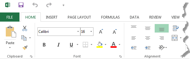
H Ribbon: To tell software what to do, you issue commands. In Excel, you can use the Ribbon to issue commands. The Ribbon is located below the Title bar. To learn more about the Ribbon, see the section The Excel Ribbon.I Formula Bar: Optionally, the Formula Bar is found below the Ribbon. Use the Formula Bar to enter and edit data. If your Formula Bar is not visible, follow the steps listed here:

Display the Formula Bar

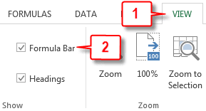
1. Choose the View tab.
2. Click Formula Bar in the Show group. Excel displays the Formula Bar.

• J Vertical and Horizontal Scroll Bars: You can move up, down, and across your window by dragging the icon located on a scroll bar. The vertical scroll bar is located along the right side of the window. The horizontal scroll bar is located just above the Status bar. To move up and down your worksheet, click and drag the icon on the vertical scroll bar up and down. To move back and forth across your workbook, click and drag the icon on the horizontal scroll bar back and forth.

• K Status Bar: The Status bar appears at the very bottom of the window and provides information such as the sum, the average, and the count of selected numbers. You can change what displays on the Status bar by right-clicking on the Status bar and selecting the options you want from the Customize Status Bar menu. A check mark next to an item means it is selected. You click an unselected menu item to select it. You click a selected menu item to unselect it.

• L Worksheet: Just below teh Formula Bar is your worksheet. This is where you enter your data. Each worksheet contains columns and rows. The columns are lettered starting wif A to Z and tan continuing wif AA, AB, AC, and so on. The rows are numbered starting wif one. Only your computer memory and your system resources limit the number of columns and rows you can have in a worksheet.

How to use the worksheet

• M Cells: Worksheets are divided into cells. The combination of a column coordinate and a row coordinate make up a cell address. You refer to cells by their cell address. For example, the cell located in the upper left corner of a worksheet is call cell A1, meaning column A, row 1. Column E10 is located under column E on row 10. You enter your data into the cells on the worksheet.

• N Normal Button : The Normal button formats your worksheet for easy data entry.

• O Page Layout Button : The Print Layout button displays your workbook in such a way as to make it easy for you to assign printing options and to see how your worksheet will look when printed.

• P Page Break Preview : The Page Break Preview button displays your workbook and shows where each page begins and ends.

• Q Zoom Slider and Zoom: The Zoom slider zooms in and out on your workbook. Dragging the slider to the left zooms out, makes your workbook smaller, and allows you to see more of your workbook. Dragging the slider to the right zooms in, makes your workbook larger, and reduces the amount of your workbook you can see. The Zoom slider appears on the Status bar if Zoom Slider is selected on the Status bar menu. The percentage of zoom appears to the right of the zoom slider, if Zoom is selected on the Status bar menu.

Advantages:

1. Sent through Emails

Excel can be sent through email and viewed by most smartphones which makes more convenient .

2. Part of Microsoft Office

Excel is a part of the Microsoft office which comes with most PC, so there is no need to purchase or install it.

3. An All in One Program

Excel is an all in one programme and does not need the addition of financial subsets.

4. Availability of Training Programs and Training Courses

There is training programs and even training courses to make users more familiar with Excel.

5. Secure

Excel files can be password protected for extra security. A user can create a password through Visual Basic programming or directly within the Excel file.[1]

6. Easy connection to OLAP

Excel is capable of connecting directly to OLAP databases and can be integrated in Pivot Tables.

Disadvantages:

1. Viruses

Viruses can be attached to an Excel file through macros. Macros are mini programs that are written into an Excel spread sheet.

2. Slow Execution

Using only one file can make the file size very big and as a result the program might run slowly.

3. Loss of Data

So you might have to break it into smaller files, by doing so their is an increased risk in Excel data being lost.

4. Hard to Use

Although there are training programs, it is still hard to use and some users might not get the hang of it.

5. Space Limit

It limits teh number of rows and columns you can use.

Installation

Removing Old or Trial Versions:

Before starting the download of Microsoft Office Professional Plus 2013, you must uninstall any old or trial versions you may still have installed on your machine. Remove the following applications:

• Old or trial versions of Microsoft Office Professional Plus 2013.
• Compatibility Pack for Office 2010.
• Any new versions that you have tried to download/install unsuccessfully.

To remove/uninstall an application:

1. Go to the Control Panel. Depending on the version of Windows you are using, choose one of the following:
   • Add/Remove Programs.
   • Uninstall a program.
2. Locate the application you want to remove.
3. Double-click the application name.
4. Follow the instructions for removing the application.

Downloading pending Windows Updates

Your current operating system (OS) must be up-to-date with Windows Updates before you can install the new software. When the updates are completed, you can install the new software.

To download pending Windows updates:

1. Click the START button.
2. Click ALL PROGRAMS.
3. Click the WINDOWS UPDATE link.
4. Download any pending updates.

32-Bit Versus 64-Bit

Both 32-bit and 64-bit options are available, but we recommend installing the 32-bit version regardless of your OS because the 32-bit option has fewer compatibility issues.

Installation instructions

Create a new workbook

• Excel documents are called workbooks. Each workbook contains one or more sheets, typically called spreadsheets. You can add as many sheets as you want to a workbook, or you can create new workbooks to keep your data separate.

• When you start excel first time (see the following picture) you can open existing workbook over here or start with a template. Since this is your first time click on the Blank workbook.

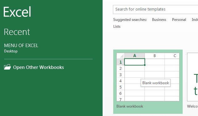
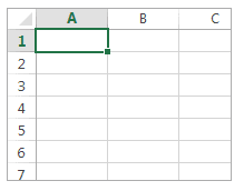
The area down here is where you create your worksheet.

Input your data

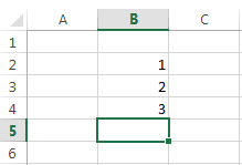
• Click an empty cell. For example, cell B2 on the below sheet.
• Type text or a number in the cell.
• Press Enter or Tab to move to the next cell.

Note : Cells are referenced by their location in the row and column on the sheet.

In the following workbook address of 1 is cell B2, 2 is cell B3, and 3 is cell B4.

Create a simple formula

Adding numbers is just one of the things you can do, but Excel can do other arithmetical formulas too. Here are some simple formulas to add, subtract, multiply or divide your numbers.

• Move the mouse in a cell and type an equal sign (=). That tells Excel that this cell will contain a formula.
• Type a combination of numbers and calculation operators, like the plus sign (+) for addition, the minus sign (-) for subtraction, the asterisk (*) for multiplication, or the forward slash (/) for the division.
  For example =(6+6*2)/3
  
• To execute the above formula Press Enter.

Note : To stay on the active cell Press Ctrl+Enter.

Apply a number format

To distinguish between different types of numbers, add a format, like currency, percentages, or dates.

• Select the cells that have numbers you want to format.
• Click Home tab –> General.
• Pick a number format

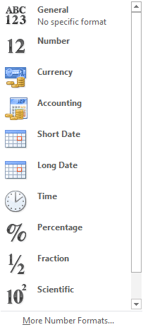
To write fraction number select “fraction”. Here is a sample worksheet with some fraction number.

Add your data use AutoSum

When you’ve entered numbers in your sheet, you can add them up to use a fast way that is AutoSum.

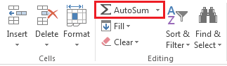
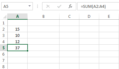
AutoSum adds up the numbers and shows the result in the cell you selected.

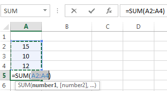
Press Enter to get desire result.

Put your data in a table

You can store a huge amount of data in a table. That lets you quickly filter or sort your data for starters.

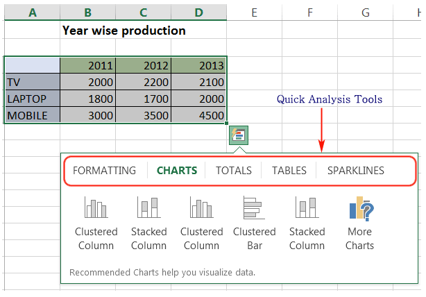
• Select your data by clicking the first cell and dragging to the cell in your data.
  To use the keyboard, hold down Shift while you press the arrow keys to select your data.
• Click the Quick Analysis button in the bottom-right corner of the selection.
  
  After clicking Quick Analysis we get the following menu then click on table button.
• 
  To filter data, uncheck the Select All box to clear all check marks, and then check the boxes of the data you want to show in your table.
• To sort the data, click Sort A to Z or Sort Z to A.

Show totals for your numbers

The Quick Analysis tools let you help to total your numbers quickly, that is the sum, average, or count whatever you want, see the picture below.

• Select the cells which contain numbers which you want to add or count.
• Click the Quick Analysis button in the right-bottom corner of the selection area.
• Then click the Total button or move your cursor across the Total button to see the calculation results for the data.

Add meaning to your data

You can see the online preview of your most important data by using conditional formatting or sparklines which highlight your valuable data for better analyzing with visualization. You can use the Quick Analysis tool for a Live Preview to try it out.

Select the data you want for your analyzing.

Click the Quick Analysis button image that appears in the right-bottom corner of your selection, shown in the picture below.

Click on Analysis Tool and get the picture below.

Click on the Formatting tab and get the options shown below.

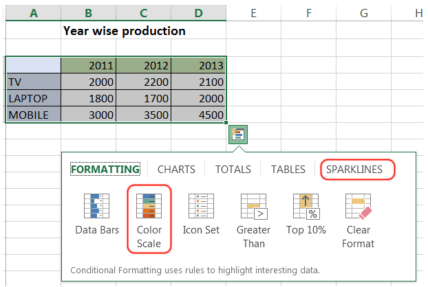
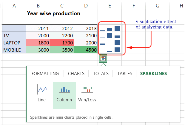
Now pick a color from Color Scale and click Sparklines and move the mouse pointer on the options and get an instant preview, shown below.

Show your data in a chart

You can use your data to convert into a chart by using Quick Analysis tool for better visual presentation in just a few clicks.

Select your data then quick analysis tool will appear at the right bottom corner of the selection area as shown in the picture below.

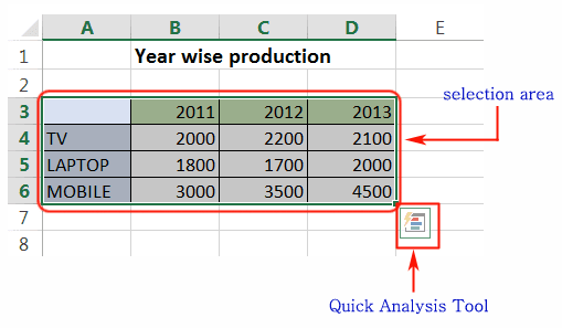
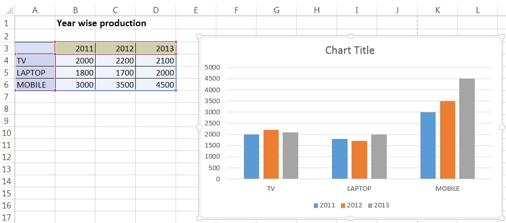
Click on Quick Analysis tool then click on Chart and move your mouse pointer on the recommended chart and see which one is your choice. See the picture below.

Click on your choice and the chart will appear in your data sheet as shown below.

Save

To save a file you can use the save button from the Quick Access Toolbar or press Ctrl+S. See the picture below.

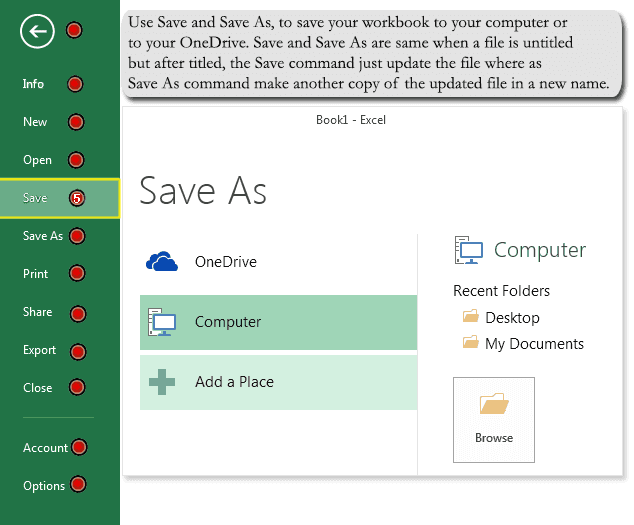
You can save the file in another way. Click File — > Save and the following screen will appear.

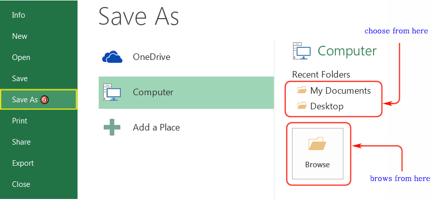
If you are saving the workbook first time the Save As window will appear and you can choose the default showing a folder for saving your workbook otherwise you can browse the folder where you want to save as shown in the above picture. Then in the file name box type the name of the file and click on Save button.

Print

Click the File –> then click Print or press Ctrl+P from the keyboard the preview window will appear.

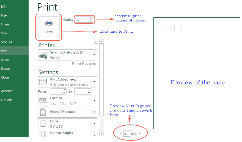
• Print preview always appears in black and white format, it depends on the printer setting.

• Page setting and printing setting can be changed by using other setting options.

• Tan click Print to print teh page.

• Once you have used to the above-mentioned features to organize your data, you can share your work with colleagues and friends in real time, which is yet another fascinating aspect of MS Excel 2013. Using the Excel WebApp, files can be shared and worked upon by others through SkyDrive. Note that if 2 people try to perform the same action on one file simultaneously, you can experience some problems.

• Moreover, if someone else is working on a Microsoft Excel worksheet, you cannot open it from SkyDrive on your device. This limitation ensures that there are no conflicting changes in the same file. However, if an Excel file that is stored online is being used by someone, you can (with permission) download or view it. But none of the changes you make will be reflected in the original file which will remain locked unless the other person closes it.

S

• Also remember that the new Excel 2013, like all other applications in Office 2013, automatically saves files to the cloud which you can access through the a browser with the Excel WebApp even if you do not have Excel on your local hard drive.

• Moving on in this Excel 2013 lesson, you can even share files via social network direct from Excel 2013. To share your files on networks like Facebook, start by saving them to SkyDrive first. If you haven’t done so, simply click “File” followed by “Share”, and then select “Invite People”. In this way, you will come across “Save As” options in a while.

• After this process, you will return back to teh Share panel where you see “Post to Social Networks”. You can choose any social network provided that it is linked with your Office 2013 account. Here you can include a message and decide whether others can edit teh worksheet you are sharing. After doing this, your post is ready to be shared.