Python Pandas Cheat Sheet: Complete Guide Tutorial For Free | CHECK-OUT

Last updated on 01st Jul 2020, Blog, Tutorials

Python Pandas Tutorial

 Pandas is an open-source, BSD-licensed Python library providing high-performance, easy-to-use data structures and data analysis tools for the Python programming language. Python with Pandas is used in a wide range of fields including academic and commercial domains including finance, economics, Statistics, analytics, etc. In this tutorial, we will learn the various features of Python Pandas and how to use them in practice.

Audience : This tutorial has been prepared for those who seek to learn the basics and various functions of Pandas. It will be specifically useful for people working with data cleansing and analysis. After completing this tutorial, you will find yourself at a moderate level of expertise from where you can take yourself to higher levels of expertise.

Prerequisites

• You should have a basic understanding of Computer Programming terminologies. A basic understanding of any of the programming languages is a plus. Pandas library uses most of the functionalities of NumPy. It is suggested that you go through our tutorial on NumPy before proceeding with this tutorial. 
• Pandas is an open-source Python Library providing high-performance data manipulation and analysis tools using its powerful data structures. The name Pandas is derived from the word Panel Data – an Econometrics from Multidimensional data.
• In 2008, developer Wes McKinney started developing pandas when in need of high performance, flexible tools for analysis of data.
• Prior to Pandas, Python was majorly used for data munging and preparation. It had very little contribution towards data analysis. Pandas solved this problem. Using Pandas, we can accomplish five typical steps in the processing and analysis of data, regardless of the origin of data — load, prepare, manipulate, model, and analyze.
• Python with Pandas is used in a wide range of fields including academic and commercial domains including finance, economics, Statistics, analytics, etc.

Key Features of Pandas

• Fast and efficient DataFrame object with default and customized indexing.
• Tools for loading data into in-memory data objects from different file formats.
• Data alignment and integrated handling of missing data.
• Reshaping and pivoting of date sets.
• Label-based slicing, indexing and subsetting of large data sets.
• Columns from a data structure can be deleted or inserted.
• Group by data for aggregation and transformations.
• High performance merging and joining of data.
• Time Series functionality.

Standard Python distribution doesn’t come bundled with Pandas modules. A lightweight alternative is to install NumPy using the popular Python package installer, pip.

Pip install pandas:

If you install Anaconda Python package, Pandas will be installed by default with the following:

Windows:

• Anaconda (from https://www.continuum.io) is a free Python distribution for SciPy stack. It is also available for Linux and Mac.
• Canopy (https://www.enthought.com/products/canopy/) is available as free as well as commercial distribution with full SciPy stack for Windows, Linux and Mac.
• Python (x,y) is a free Python distribution with SciPy stack and Spyder IDE for Windows OS. (Downloadable from http://python-xy.github.io/)

Linux: Package managers of respective Linux distributions are used to install one or more packages in SciPy stack.

For Ubuntu Users:

For Fedora Users:

Pandas deals with the following three data structures:

• Series
• DataFrame
• Panel

These data structures are built on top of Numpy arrays, which means they are fast.

Dimension & Description:

The best way to think of these data structures is that the higher dimensional data structure is a container of its lower dimensional data structure. For example, DataFrame is a container of Series, Panel is a container of DataFrame.

Data Structure	Dimensions	Description
Series	1	1D labeled homogeneous array, size immutable.
Data Frames	2	General 2D labeled, size-mutable tabular structure with potentially heterogeneously typed columns.
Panel	3	General 3D labeled, size-mutable array.

Building and handling two or more dimensional arrays is a tedious task, and a burden is placed on the user to consider the orientation of the data set when writing functions. But using Pandas data structures, the mental effort of the user is reduced.

For example, with tabular data (DataFrame) it is more semantically helpful to think of the index (the rows) and the columns rather than axis 0 and axis 1.

Mutability:

All Pandas data structures are value mutable (can be changed) and except Series all are size mutable. Series is size immutable.

Note : DataFrame is widely used and one of the most important data structures. Panel is used much less.

Series:

Series is a one-dimensional array-like structure with homogeneous data. For example, the following series is a collection of integers 10, 23, 56, …

10

23

56

17

52

61

73

90

26

72

Key Points:

• Homogeneous data
• Size Immutable
• Values of Data Mutable

DataFrame:

DataFrame is a two-dimensional array with heterogeneous data. For example,

Name	Age	Gender	Rating
Steve	32	Male	3.45
Lia	28	Female	4.6
Vin	45	Male	3.9
Katie	38	Female	2.78

The table represents the data of a sales team of an organization with their overall performance rating. The data is represented in rows and columns. Each column represents an attribute and each row represents a person.

Data Type of Columns:

The data types of the four columns are as follows :

Column	Type
Name	String
Age	Integer
Gender	String
Rating	Float

Key Points:

• Heterogeneous data
• Size Mutable
• Data Mutable

Panel:

Panel is a three-dimensional data structure with heterogeneous data. It is hard to represent the panel in graphical representation. But a panel can be illustrated as a container of DataFrame.

Key Points:

• Heterogeneous data
• Size Mutable
• Data Mutable

Series is a one-dimensional labeled array capable of holding data of any type (integer, string, float, python objects, etc.). The axis labels are collectively called indexes.

pandas.Series

A pandas Series can be created using the following constructor:

The parameters of the constructor are as follows:

Parameter	Description
Data	data takes various forms like ndarray, list, constants
Index	Index values must be unique and hashable, same length as data. Default np.arange(n) if no index is passed.
Dtype	dtype is for data type. If None, data type will be inferred
Copy	Copy data. Default False

A series can be created using various inputs like :

• Array
• Dict
• Scalar value or constant

Create an Empty Series:

A basic series, which can be created is an Empty Series.

Example

Its output is as follows −

Create a Series from ndarray:

If data is an ndarray, then index passed must be of the same length. If no index is passed, then by default index will be range(n) where n is array length, i.e., [0,1,2,3…. range(len(array))-1].

Example 1

Its output is as follows:

dtype: object

We did not pass any index, so by default, it assigned the indexes ranging from 0 to len(data)-1, i.e., 0 to 3.

Example 2

Its output is as follows −

We passed the index values here. Now we can see the customized indexed values in the output.

Create a Series from dict:

A dict can be passed as input and if no index is specified, then the dictionary keys are taken in a sorted order to construct the index. If the index is passed, the values in data corresponding to the labels in the index will be pulled out.

Example 1

Its output is as follows:

Observe: Dictionary keys are used to construct indexes.

Example 2

Its output is as follows −

Create a Series from Scalar:

If data is a scalar value, an index must be provided. The value will be repeated to match the length of index

Its output is as follows −

Accessing Data from Series with Position:

Data in the series can be accessed similar to that in an ndarray.

Example 1

Retrieve the first element. As we already know, the counting starts from zero for the array, which means the first element is stored at zeroth position and so on.

Its output is as follows :

Example 2

Retrieve the first three elements in the Series. If a : is inserted in front of it, all items from that index onwards will be extracted. If two parameters (with : between them) is used, items between the two indexes (not including the stop index)

Its output is as follows :

Example 3

Retrieve the last three elements.

Its output is as follows :

Its output is as follows:

Retrieve Data Using Label (Index):

A Series is like a fixed-size dict in that you can get and set values by index label.

Example 1

Retrieve a single element using index label value.

Example 2

Retrieve multiple elements using a list of index label values.

Its output is as follows :

Example 3

If a label is not contained, an exception is raised.

Its output is as follows:

A Data frame is a two-dimensional data structure, i.e., data is aligned in a tabular fashion in rows and columns.

Features of DataFrame:

• Potentially columns are of different types
• Size – Mutable
• Labeled axes (rows and columns)
• Can Perform Arithmetic operations on rows and columns

Structure:

Let us assume that we are creating a data frame with student’s data.

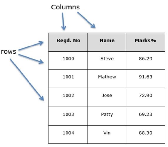
You can think of it as an SQL table or a spreadsheet data representation.

pandas.DataFrame:

A pandas DataFrame can be created using the following constructor.

pandas.DataFrame( data, index, columns, dtype, copy)

Conclusion:

Early Access puts eBooks and videos into your hands whilst they’re still being written, so you don’t have to wait to take advantage of new tech and new ideas.