Top [ 45+ ] Excel Interview Questions & Answers [LATEST]

Last updated on 03rd Jun 2020, Blog, Interview Questions

Advanced Excel refers to the capabilities and functionalities of the Microsoft Excel application that enable the user to execute intricate calculations, analyze massive amounts of data, conduct data analysis, and show data more effectively, among other things.Given how important time is in the business world, advanced Excel training may be quite beneficial for your business and career.

1. Explain about MS Excel

Ans: 

Microsoft Excel is a robust and popular spreadsheet program that enables users to effectively organize, analyze, and modify data. Users are given a grid-like workspace with rows and columns where they may enter textual or numeric data into cells. Excel has a variety of tools for building sophisticated formulae, doing data analysis, producing charts and graphs, and creating pivot tables for summing up data. Excel’s power extends beyond simple arithmetic calculations.

2. What do you mean by cells in an Excel sheet?

Ans: 

In an Excel sheet, a cell refers to a single intersection point within the grid-like structure formed by rows and columns. Each cell is identified by a unique combination of a column letter and a row number, such as “A1” or “B3”. Cells are the fundamental units where you can input, store, and manipulate data.

3. Explain what is a spreadsheet?

Ans: 

A spreadsheet is a digital document or application that is used to structurely organise, store, and manipulate data. It is made up of a grid of rows and columns, with each intersection forming a cell. Spreadsheets are frequently used for data entry, calculations, analysis, and visualisation.

4. What do you mean by cell address?

Ans: 

A cell address in a spreadsheet refers to a unique identifier for a specific cell within the grid of rows and columns. It makes it easier for you to locate a cell’s precise placement inside the spreadsheet. The cell address is typically a combination of a column letter and a row number.

5. Can you add cells?

Ans: 

Right-click on the row number or column letter where you want to insert cells. Then, select the “Insert” option from the context menu. This will shift the existing data down (for rows) or to the right (for columns) to make space for the new cells.

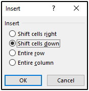
Select the desired option and then click on OK.

6. Can you format MS Excel cells? If yes, then how?

Ans: 

Yes, you can format cells in Microsoft Excel to control how data is displayed, enhance readability, and emphasize important information. Formatting options include adjusting font styles, colors, number formats, alignment, and more.

7. Can you add comments to a cell?

Ans: 

Yes, you may add comments to a cell in Microsoft Excel. Comments are used to offer extra information, clarifications, or notes concerning the content of a single cell. When you make a comment to a cell, a little indication appears in the cell’s corner, and the comment itself is displayed when you hover over the cell.

8. Can you add new rows and columns to an Excel sheet?

Ans: 

Yes, you can expand or reorganise your data on an Excel sheet by adding additional rows and columns. Adding rows and columns might assist your spreadsheet’s layout change or accommodate more data.

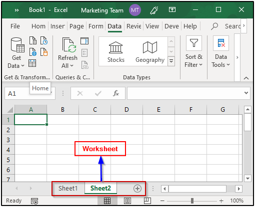
9. What is a Ribbon and where does it appear?

Ans: 

The Ribbon is a graphical user interface component included in Microsoft Office applications such as Excel, Word, and PowerPoint.The Ribbon is located directly below the title bar at the top of the programme window. It is divided into several tabs, each representing a different category of functions. When you click a tab, it shows a group of linked instructions and settings.

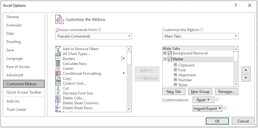
You can select or unselect any option of your choice from here.

10. How do you freeze panes in Excel?

Ans: 

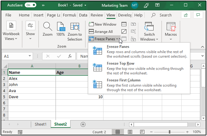
To Freeze Rows and Columns: If you wish to freeze both rows and columns, choose the cell that is immediately below the desired row and immediately to the desired column’s right.

To Freeze Only Rows: If you want to freeze only rows, select the cell just below the row you want to freeze.

To Freeze Only Columns: If you want to freeze only columns, select the cell just to the right of the column you want to freeze.

11. How do you insert a Note into a cell?

Ans: 

• Decide the cell you wish to insert the note into.
• The “Review” tab is located in the Excel ribbon.
• Under the “Comments” section, click the “New Comment” button. If you right-click the cell, you can also choose “Insert Comment” from the menu.
• The cell will be surrounded by a tiny text box. In this area, put any notes or comments you like to make.
• If necessary, drag the border of the comment box to resize it.
• When you right-click the comment box, formatting choices are also presented to you.

12. Can you protect workbooks in Excel?

Ans: 

Yes, you can protect workbooks in Excel to prevent unauthorized access, changes to certain elements, or modifications to the structure of the workbook.

13. How do you apply the same format to all of the sheets in a workbook?

Ans: 

Applying the same format to all sheets in an Excel workbook can be achieved using a feature called “Cell Styles.” Cell Styles allow you to define and apply consistent formatting to cells across multiple sheets.

14. What do you understand by Relative Cell Addresses?

Ans: 

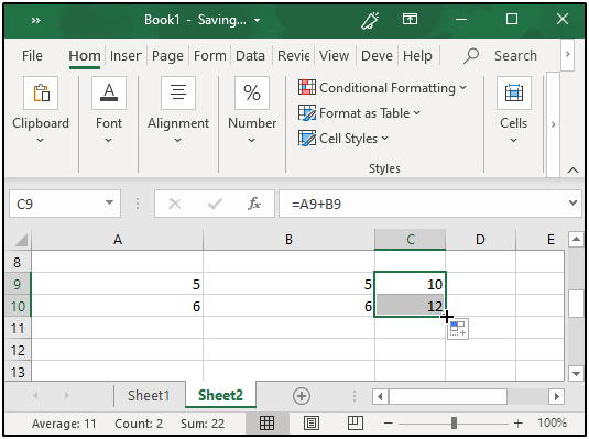
Relative cell addresses refer to the way Excel references cells in formulas when you copy or fill them to other cells. In a relative reference, the cell address is adjusted automatically based on its position relative to the original cell when the formula is copied or filled to another cell.

15. What should you do if you don’t want the copied cell addresses to be changed?

Ans: 

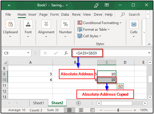
 If you don’t want the copied cell addresses to be changed when you copy or fill formulas to other cells, you can use absolute cell references or mixed cell references. Absolute cell references lock the cell address so that it doesn’t change when the formula is copied or filled, while mixed cell references lock either the row or column part of the cell address.

16. What will you do if either the column letter or the row number, but not both, has to be changed?

Ans: 

Determine Which Part to Lock: Decide whether you want to lock the column letter or the row number while allowing the other part to change.

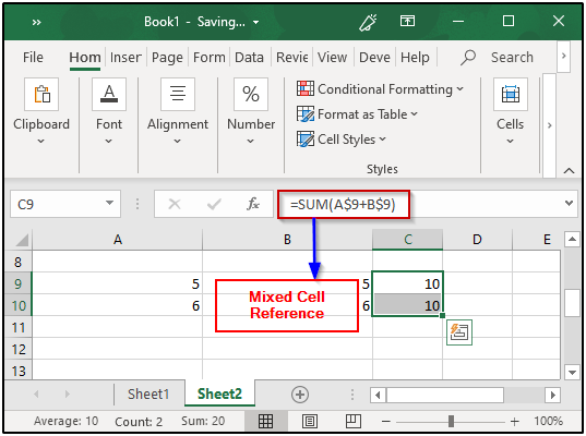
Mixed Cell Reference Format: To lock the column while allowing the row to change, place a dollar sign ($) before the column letter but not before the row number. 

To lock the column (e.g., column A) while allowing the row to change: $A1

To lock the row (e.g., row 1) while allowing the column to change: A$1

Using the Mixed Reference: Insert the mixed reference into your formula wherever you need to reference the cell. 

17. Can you protect the cells of a sheet from being copied?

Ans: 

Yes, you can protect cells in an Excel sheet from being copied or accessed by applying worksheet protection. Worksheet protection allows you to control various actions that users can perform on the sheet, including copying, formatting, and more.

18. How do you create Named Ranges?

Ans: 

Select Cells: The cell or range of cells you want to name should be selected.

Name Box: Locate the Name Box on the left side of the formula bar. It typically displays the cell address, such as “A1” or “B2.”

Enter Name: Click in the Name Box and enter the desired name for the range, without spaces. The name can’t start with a number or include special characters except underscores (_).

Press Enter: After entering the name, press “Enter.”

19. What are macros?

Ans: 

 Macros in Excel are sets of recorded or manually programmed actions that can be played back to automate repetitive tasks. They allow you to perform a sequence of actions with a single command, making complex or time-consuming tasks more efficient and consistent. Macros can involve actions like data manipulation, formatting, calculations, and more.

20. How do you create dropdown lists in Excel?

Ans: 

Select the Cell(s): To construct a drop-down menu, click on the cell or cells you wish to use.

Data Tab: Go to the “Data” tab on the Ribbon.

Data Validation: Click on the “Data Validation” button in the “Data Tools” group. Go to the “Settings” tab in the Data Validation dialog box that displays.

Allow: Choose “List” from the “Allow” dropdown menu.

Source: In the “Source” box, enter the list of options you want in your drop-down

21. Explain Pivot tables along with their features.

Ans: 

A pivot table is a strong Excel feature that makes it simple and quick to summarise and analyze vast volumes of data. It facilitates the creation of dynamic tables that may be adjusted, sorted, filtered, and computed in order to turn raw data into insightful understandings.

Features of Pivot Tables:

• Data Summarization
• Drag-and-Drop Interface
• Dynamic Updates
• Filters
• Sorting and Grouping
• Calculated Fields and Items

22. How do you create Pivot Tables?

Ans: 

• Prepare Your Data
• Select Your Data
• Insert Pivot Table
• Choose Data Range
• Choose Destination
• Pivot Table Field List
• Drag and Drop Fields
• Customize and Format
• Update and Refresh

23. What are Pivot charts in MS Excel?

Ans: 

Pivot Charts in Microsoft Excel are visual representations of data that are dynamically linked to Pivot Tables. They allow you to visualize and explore summarized data from Pivot Tables in the form of charts and graphs. Pivot Charts offer a powerful way to analyze and present data trends, patterns, and comparisons.

24. Can you create Pivot tables using multiple tables?

Ans: 

• Click anywhere within one of the tables you’ve created.
• Select “PivotTable” from the “Tables” group on the “Insert” tab of the Ribbon. You’ll see the “Create PivotTable” dialog box.
• Ensure that the “Choose multiple tables” option is selected.
• Select the tables you want to include in the Pivot Table by checking the boxes.
• Click “OK.”

25. What happens when you check the Defer Layout Update option present in the PivotTable Fields window?

Ans: 

When the “Defer Layout Update” checkbox is selected in Excel’s PivotTable Fields panel, the Pivot Table is temporarily prevented from updating and rearranging the layout while you make changes to the fields. This can be useful when you want to make multiple changes to the Pivot Table’s structure before applying the updates.

26. Can a pivot table be made from a table from a separate worksheet?

Ans: 

Yes, you can create a Pivot Table using data from a table located in a separate worksheet within the same Excel workbook. Excel allows you to reference data from other worksheets when creating Pivot Tables, making it convenient to analyze and summarize data stored in different sheets.

27. Can you see the specifics of the results shown in a pivot table?

Ans: 

Yes, you can create a Pivot Table using data from a table located in a separate worksheet within the same Excel workbook. Excel allows you to reference data from other worksheets when creating Pivot Tables, making it convenient to analyze and summarize data stored in different sheets. 

28. How can data be filtered using pivot tables?

Ans: 

Pivot Tables in Excel allow you to filter data so that you may concentrate on particular subsets of data, making it simpler to analyse and display pertinent facts. With the use of pivot tables, you may filter data in a variety of ways to focus your study on a few key factors.

29. How do you change the value field to show some other result other than the Sum?

Ans: 

In a Pivot Table, you may edit the value field to display results other than the sum by applying other summary functions such as average, count, minimum, maximum, and so on. This allows you to analyse your data in a variety of ways. 

30. How to stop automatic sorting in PivotTables?

Ans: 

Open the PivotTable and identify the field for which you want to retain the existing order. Right-click on a cell within the column of that field and access “Field Settings.” In the “Layout & Print” tab of the dialog box, uncheck the “Automatic” option under “Sort.” Click “OK” to save the changes.

31. What do you understand about Excel functions?

Ans: 

Excel functions are predefined formulas that perform specific calculations, operations, or tasks in Microsoft Excel. They enable users to easily carry out a variety of actions on their data since they are made to streamline numerous processes and simplify difficult computations. Excel functions take inputs (arguments) and return results based on those inputs.

32. What are the various categories of functions available in Excel?

Ans: 

• Math and Trigonometry
• Statistical
• Logical
• Text
• Date and Time
• Financial

33. What is the operator precedence of formulas in Excel?

Ans: 

 Operator precedence in Excel refers to the order in which mathematical and logical operations are evaluated within a formula. Just like in mathematics, Excel follows a set of rules to determine which operations should be performed first when a formula contains multiple operators.

34. Explain SUM and SUMIF functions.

Ans: 

SUM Function: The SUM function is one of the most basic and frequently used functions in Excel. It’s used to calculate the sum (total) of a range of numbers. You provide a range of cells, and the SUM function adds up the values within that range.

SUMIF Function: The SUMIF function computes the sum of values in a range based on a predefined condition. It’s useful when you want to sum values that meet certain criteria.

35. What is a Scenario Manager?

Ans: 

A Scenario Manager in Microsoft Excel is a tool that allows you to design and manage multiple scenarios for a spreadsheet model. A scenario is a set of input values that you may construct and store to easily compare alternative outcomes or results.

36. How is the percentage determined in Excel?

Ans: 

• You can format a cell to display its value as a percentage without changing the actual value stored in the cell.
• To format a cell, select a range of cells.
• Right-click and choose “Format Cells” from the context menu, or go to the “Home” tab on the Ribbon and use the “Format Cells” option.
• Navigate to the “Number” tab in the “Format Cells” dialog box.
• Choose the “Percentage” category and specify the desired number of decimal places.
• Click “OK” to apply the formatting.

37. How do you compute compound interest in Excel?

Ans: 

The FV function uses a sequence of regular deposits, compound interest, and a fixed interest rate to determine the future value of an investment. The Syntax is :

FV(rate, nper, pmt, [pv], [type])

38. In Microsoft Excel, how do you find averages?

Ans: 

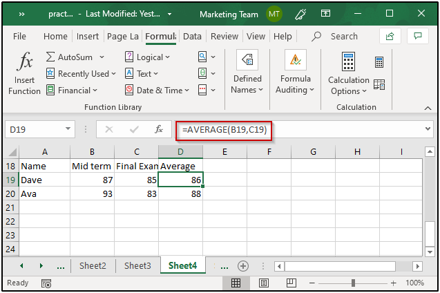
The FV function determines the future value of an investment using a sequence of regular deposits, compounding interest, and a fixed interest rate. 

AVERAGE(number1, [number2], …)

EXAMPLE:

39. What is VLOOKUP in Excel?

Ans: 

It is used to find a certain value in the first column of a table or range and then obtain a related value from another column inside the same row. VLOOKUP is very handy when dealing with enormous datasets and needing to rapidly discover and extract information based on a specified set of criteria.

40. How does the VLOOKUP function work?

Ans: 

The Excel VLOOKUP function, which stands for “Vertical Lookup,” finds a certain value in the first column of a chosen range or table and then retrieves a relevant value from a chosen column in the same row. For swiftly locating and extracting data based on a specified criterion, this tool is quite helpful.

41. Explain the exact match

Ans: 

An exact match in the context of the VLOOKUP function refers to finding a value in a data range that matches the lookup value precisely. In other words, the lookup value you provide is expected to be found exactly as it is in the first column of the specified data range.

42. Explain the approximate match

Ans: 

The nearest value inside a data range that is less than or equal to the lookup value is referred to as an approximate match in the context of the VLOOKUP function. When working with numerical data, this kind of match is frequently used to locate the value that is most pertinent to a given criterion, such as locating a price that corresponds to a specified amount within a pricing list.

43. Can you use VLOOKUP for multiple tables?

Ans: 

Yes, by combining various functions and strategies, you may utilise the VLOOKUP function to do lookups across many tables. Using the IFERROR function in combination with several VLOOKUP functions is a typical strategy.

44. How do you perform a horizontal lookup in Excel?

Ans: 

In Excel, performing a horizontal lookup is also known as an “HLOOKUP,” which stands for “Horizontal Lookup.” Like the VLOOKUP function, the HLOOKUP function searches for a specific value in the first row of a table or range and retrieves a related value from a different row within the same column.

45. How will you fetch the current date in Excel?

Ans: 

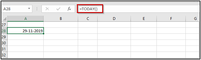
The TODAY function in Excel may be used to retrieve the current date. The TODAY function produces a serial number representing the current date, which you may later convert as a date using the format of your choice.

Enter the following formula:

TODAY()

EXAMPLE:

46. How does the AND function work?

Ans: 

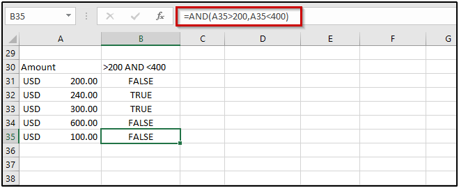
The AND function in Excel is a logical function that allows you to test multiple conditions and determine whether all of them are true. It returns TRUE if all the specified conditions are true, and FALSE if at least one condition is false. The AND function is particularly useful when you want to perform complex logical tests involving multiple criteria.

SYNTAX:

EXAMPLE:

47. What exactly is the What If Analysis?

Ans: 

“What-If Analysis” in Excel refers to a set of tools and techniques that allow you to explore different scenarios by changing input values and observing the resulting outcomes. It’s a powerful feature that helps you understand how changes to variables can affect calculations, formulas, and overall results in your spreadsheet. 

48. Can you make shortcuts for the formulas that are utilized the most?

Ans: 

Yes, you may utilize Excel’s “Customize Ribbon” tool to set up unique keyboard shortcuts for commonly used formulae. Although you can’t naturally attach keyboard shortcuts to individual formulae in Excel, you can make a custom tab on the Ribbon with buttons that are tied to your most often-used formulas. Then, you may rapidly retrieve those formulae by pressing Alt + [Number].

49. In Excel, what distinguishes formulas from functions?

Ans: 

Formulas: A formula in Excel is an equation that you create to perform calculations using cell references, values, operators, and functions. Formulas can involve simple arithmetic operations like addition, subtraction, multiplication, and division, as well as more complex calculations and logical operations.

Functions: A function in Excel is a predefined operation that performs a specific task, such as calculations, data analysis, text manipulation, and more. Functions are built-in features of Excel and have specific names (e.g., SUM, AVERAGE, IF) followed by parentheses that contain arguments (inputs) to the function. 

50. How do you use wildcards with VLOOKUP?

Ans: 

In Excel, you can use wildcards with the VLOOKUP function to perform approximate matches based on patterns or partial text. Wildcards are special characters that represent unknown or variable values. The two commonly used wildcards are the asterisk * and the question mark ?

51. What are the different data formats in Excel?

Ans: 

Different data formats allow you to control the appearance of your data and ensure that it is correctly understood by Excel for calculations and analysis. 

• Number Formats
• Text Formats
• Date and Time Formats
• Special Formats
• Custom Formats
• Accounting Formats
• Conditional Formats

52. How can you wrap text in Excel?

Ans: 

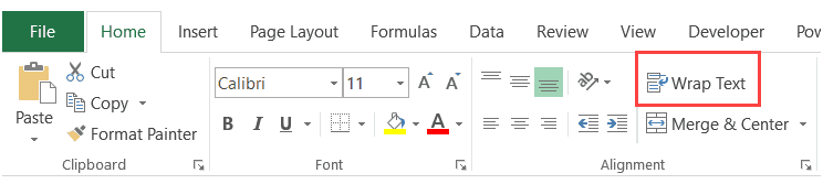
 In Excel, wrapping text allows you to display cell contents on multiple lines within a single cell, so that all the text fits within the cell’s width. This is particularly useful when you have lengthy text or when you want to make your data more readable without adjusting column widths.

53. How can you merge cells in Excel?

Ans: 

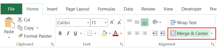
• Choose the cells that you wish to combine. These cells ought to be close neighbours, either in a row or a column.
• On the Ribbon, select the “Home” tab.
• The “Merge & Centre” menu button is found in the “Alignment” category. To view the dropdown menu, press the button.

54. What is ‘Format Painter’ used for?

Ans: 

Excel’s “Format Painter” is an effective tool that enables you to swiftly replicate the formatting (including font styles, cell colors, borders, and more) to another cell or range of cells from one cell or range of cells. It’s especially helpful if you want to keep a uniform formatting style throughout your worksheet’s various sections.

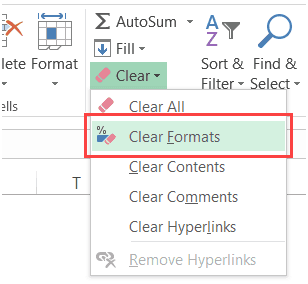
55. How would you clear all the formatting without removing the cell contents?

Ans: 

To remove all formatting from a cell or group of cells in Excel without deleting the cell contents, use the “Clear Formats” option.This will reset the formatting of the selected cells to the default formatting while preserving the data within the cells.

56. What is conditional formatting?

Ans: 

 Conditional formatting is a feature in Excel that allows you to automatically apply formatting (such as font color, cell background color, and more) to cells based on specific conditions or rules. It’s a powerful tool that helps you visually highlight and analyze data by emphasizing patterns, trends, and exceptions in your worksheet. Conditional formatting makes it easier to spot important information at a glance.

57. How would you highlight cells with negative values in it?

Ans: 

• Go to the “Home” tab on the Ribbon.
• Click the “Conditional Formatting” dropdown arrow in the “Styles” group, and then select “New Rule.”
• Within the “New Formatting Rule” dialog box’s “Select a Rule” section is where you may find the “Format cells that contain” option.
• In the “Format cells that contain” section, select “Cell Value” in the first dropdown, “less than” in the second dropdown, and enter 0 in the third field to specify that you want to highlight negative values.
• Click the “Format” button to configure the formatting for cells containing negative values. For example, you can choose a red font color or a red cell fill color.
• After setting up the formatting style, click “OK” to apply the rule.
• You’ll be returned to the “New Formatting Rule” dialog box. You can preview how the rule will affect your selected cells in the “Preview” section. If you’re satisfied, click “OK” to apply the conditional formatting.

58. How would you indicate which cells have duplicate values?

Ans: 

• Choose the cell range or individual cells that contain the duplicate values you want to find and highlight.
• On the Ribbon, select the “Home” tab.
• In the “Styles” section, click the “Conditional Formatting” dropdown arrow and then choose “New Rule.”
• Under “Select a Rule Type” in the “New Formatting Rule” dialog box, select “Format cells that contain.”
• Choose “Duplicate” from the first choice in the “Format cells that contain” section.
• To set the formatting for cells with duplicate values, click the “Format” button. For instance, you might select a backdrop color to draw attention to duplicate cells.
• To apply the rule after configuring the formatting style, click “OK”.

59. How would you highlight cells with errors in it?

Ans: 

• Choose the cell range or individual cells that you want to detect and indicate as having mistakes.
• On the Ribbon, select the “Home” tab.
• In the “Styles” section, click the “Conditional Formatting” dropdown arrow and then choose “New Rule.”
• Under “Select a Rule Type” in the “New Formatting Rule” dialog box, select “Format cells that contain.”
• Choose “Errors” from the first selection in the “Format cells that contain” section.
• To change the formatting for cells that contain mistakes, click the “Format” button. For instance, you may select a backdrop color to draw attention to cells that contain mistakes.
• To apply the rule after configuring the formatting style, click “OK”.

60. How can you make text invisible in Excel?

Ans: 

In Excel, you cannot make text completely invisible, but you can hide it using a font color that matches the cell background color. This will effectively render the text “invisible” because it will blend into the background.

61. What order of operations does Excel utilize to evaluate formulas?

Ans: 

Microsoft Excel follows a specific order of operations, often referred to as the “order of operations” or “precedence rules,” to evaluate formulas. 

The following is Excel’s order of operations:

• Parentheses
• Exponents
• Multiplication and Division
• Addition and Subtraction
• Concatenation

62. How do functions and formulas in Excel differ from one another?

Ans: 

 In essence, functions are pre-built tools that can simplify complex calculations and data manipulation tasks by encapsulating specific operations. Formulas, on the other hand, are expressions you create using operators, cell references, and functions to achieve your desired calculations and manipulations.

63. What are the best five functions in Excel, in your opinion?

Ans: 

SUM: A range of values can be added up using the SUM function.

IF: Conditional computations are possible using the IF function. 

VLOOKUP: This function locates a value in a table and retrieves a corresponding value from a different column. 

INDEX-MATCH: Although it is not a single function, the INDEX and MATCH combination is a strong substitute for VLOOKUP.

AVERAGE: The AVERAGE function determines the mean of a range of data. 

64. What differentiates absolute from relative cell references?

Ans: 

In Microsoft Excel, cell references play a pivotal role in creating dynamic and adaptable formulas. Two primary types of references—absolute and relative—serve distinct purposes in formula construction. 

Relative Cell References: In a relative reference, only the column and row positions are considered relative to the formula’s position.In this example, if you duplicate the formula =A1 + B1 from cell C1 to cell C2, C2 will immediately change to =A2 + B2.

Absolute Cell References: In contrast, an absolute cell reference remains constant regardless of where the formula is copied or filled. For example, if you have the formula =$A$1 + B1 in cell C1 and you copy it to cell C2, the formula in C2 will still be =$A$1 + B1, without any adjustments to the references.

65. What are the many types of Excel errors?

Ans: 

• DIV/0! (Divide by Zero Error)
• VALUE! (Value Error)
• NUM! (Number Error)
• NULL! (Intersection Error)
• REF! (Reference Error)
• DATE! (Date Error)
• TEXT! (Text Error)

66. How may errors be fixed while using Excel formulas?

Ans: 

Identify the Error: Look for the error message (e.g., #DIV/0!, #VALUE!, #N/A) in the formula cell. This indicates the type of error you’re dealing with.

Review Formula: Carefully review the formula for typos, incorrect references, or mathematical errors that could be causing the problem.

Use Error Handling: Employ error handling functions like IFERROR or IFNA to provide alternate outputs or messages when errors occur.

Check Data and Logic: Verify the data being used in the formula and ensure logical consistency, such as avoiding divide-by-zero situations or improper data types.

67. Which Excel function would you use to retrieve the current date and time?

Ans: 

Using Excel’s NOW() function, you may get the current date and time. Every time the worksheet is recalculated, the NOW() method updates the value it provides with the current date and time.

68. How can you use a formula to merge the text from various cells?

Ans: 

To combine text from many cells into one, you may use Excel’s CONCATENATE() function or the ampersand (&) operator. You can combine text using either the & operator or the CONCATENATE() function, depending on which way feels most natural to you.

69. How would you calculate the length of a text string stored in a cell?

Ans: 

The length of a text string contained in a cell may be found using Excel’s LEN() function. The LEN() function returns the whole text string’s character count, including spaces and special characters.

70. What is the syntax for the VLOOKUP function?

Ans: 

To find a value in the first column of a range and return a similar value in the same row from a specified column, utilise Excel’s VLOOKUP function. The syntax is:

VLOOKUP(lookup_value, table_array, col_index_num, [range_lookup])

71. How do you remove leading, trailing, and double spaces from text in Excel?

Ans: 

With the TRIM() function, leading and trailing spaces are eliminated from text strings, leaving just a single space between words.

Syntax:TRIM(text)

Using SUBSTITUTE() to Remove Double Spaces: The SUBSTITUTE() function may be used to swap out double spaces for single spaces in a text string.

Syntax:SUBSTITUTE(text, old_text, new_text)

Types of Additional Spaces

You may use the TRIM() and SUBSTITUTE() methods in a calculation to eliminate any excess spaces, including leading, trailing, and double spaces:

TRIM(SUBSTITUTE(SUBSTITUTE(A1, ”  “, ” “), CHAR(160), ” “))

72. What VLOOKUP function drawbacks are now recognized?

Ans: 

Inflexibility with Column Insertions/Deletions: If you insert or delete columns within the table_array, the col_index_num argument may become invalid, leading to incorrect results.

Slower Performance with Large Data: VLOOKUP can be slower when working with large datasets, as it searches through data sequentially. Other functions like INDEX-MATCH may offer better performance in such cases.

Limited to One Lookup Column: Only the first column of the table_array may be used for VLOOKUP searches. If you need to search across multiple columns, you need to use multiple VLOOKUP functions or another approach.

Lack of Context Sensitivity: VLOOKUP doesn’t provide the flexibility to take into account additional factors or conditions when performing the lookup, which might be needed in some scenarios.

73. When would you apply the SUBTOTAL function?

Ans: 

In Excel, the SUBTOTAL function is used to add, subtract, multiply, divide, and total a range of data while, at the user’s discretion, disregarding hidden rows and mistakes. You may compute different summary statistics or carry out computations while taking into account only the visible rows when dealing with filtered or subtotaled data, which is quite beneficial.

74. What do “volatile functions” mean? Give me a few examples.

Ans: 

 In Excel, “volatile functions” are functions that recalculate anytime there is a workbook update, whether or not the change changes the function’s inputs. The performance of your Excel worksheet can be greatly impacted by these functions, particularly when working with huge datasets or intricate calculations, which is why they are regarded as volatile.

NOW(): Returns the current date and time. Since the current date and time are always changing, this function recalculates frequently.

TODAY(): Returns the current date. Similar to NOW(), this function recalculates whenever the date changes.

75. Which keyboard shortcuts do you find most helpful?

Ans: 

• Ctrl + C: Copy selected text or items to the clipboard.
• Ctrl + X: Cut selected text or items to the clipboard.
• Ctrl + V: Paste the contents of the clipboard.
• Ctrl + Z: Undo the last action.
• Ctrl + Y: Redo the last undone action.

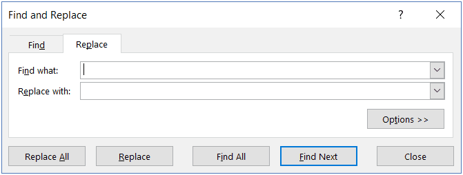
76. What is the shortcut for activating the find and replace dialog box?

Ans: 

Pressing Ctrl + H simultaneously will open the “Find and Replace” dialog box, allowing you to search for specific text and replace it with another text throughout the document or selected range. This shortcut can be very handy when you need to perform multiple find and replace operations quickly.

77. What is the keyboard shortcut for opening a new Excel workbook?

Ans: 

• Ctrl + N: Opens a new blank workbook.
• Ctrl + T: Opens a new tab in the Excel window, resulting in the creation of a new workbook.

78. How do you select every cell on the worksheet?

Ans: 

Pressing Ctrl + A simultaneously will select all cells on the active worksheet. This shortcut is a quick way to highlight and work with all the cells in your data. Keep in mind that if you have filtered data, only the visible cells will be selected using this shortcut. If you want to select all cells, including hidden ones, you would first need to clear the filter.

79. How would you add another line to the same cell?

Ans: 

Using the “Alt + Enter” keyboard shortcut in Excel, you may add another line to the same cell. This shortcut inserts a line break within the content of the cell, allowing you to begin a new line of text without travelling to the next cell.

80. What is the Excel shortcut for inserting a comment?

Ans: 

The Excel shortcut for inserting a comment is Shift + F2.

81. How and when would you utilize a pivot table?

Ans: 

The pivot table feature in Excel is a powerful tool that enables manipulating and analysing large data sets easy and versatile. You might utilise a pivot table while working with massive datasets that require summarization, comparison, and pattern detection.

82. What do the different Pivot Table parts consist of?

Ans: 

A Pivot Table in Excel consists of several key parts that allow you to organize, summarize, and analyze your data effectively. These parts include:

Pivot Table Fields List or Field List: This panel normally appears when you construct a pivot table on the right side of the Excel window. It lists all the column headers (fields) from your source data.

Row Labels Area: This area is located on the left side of the pivot table. It holds the fields that you want to use as row labels, organizing data vertically. 

Column Labels Area: Positioned above the pivot table, this area holds the fields that you want to use as column labels. 

Values Area: This area is at the center of the pivot table. It holds the fields that you want to summarize, such as calculating sums, averages, counts, etc. 

Report Filter Area: Positioned above the pivot table or to the left, this area allows you to apply filters to the entire pivot table.

83. What exactly are slicers?

Ans: 

Slicers in Excel are interactive visual filters that provide a user-friendly way to filter data in pivot tables and pivot charts. They are graphical buttons that allow you to quickly filter data by selecting specific items from a field, making it easier to analyze and explore data dynamically. 

84. Explain a pivot chart.

Ans: 

 A pivot chart in Excel is a visual depiction of the data from a pivot table. You may use many chart kinds, including bar charts, line charts, pie charts, and more, to visualize and evaluate compiled data. Due to the fact that they both derive their information from the same underlying data source, pivot charts and pivot tables are closely related. 

85. What differentiates pivot charts from standard charts?

Ans: 

Here are the key differences between pivot charts and standard charts:

Data Source:

Pivot Charts: Pivot charts are based on pivot tables. The data displayed in a pivot chart is derived from the summarized and aggregated data in the associated pivot table. 

Standard Charts: Standard charts are based on a selected range of data within a worksheet.

Flexibility:

Pivot Charts: Pivot charts are more dynamic and flexible. 

Standard Charts: Standard charts are less flexible.

Interactivity:

Pivot Charts: Pivot charts are inherently interactive due to their connection with pivot tables

Standard Charts: Standard charts are static and lack the interactive features provided by pivot charts. 

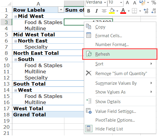
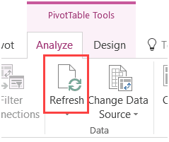
86. How is a pivot table refreshed?

Ans: 

• Right-click any cell within the pivot table.
• From the context menu, select “Refresh.”

87. Can dates be organized in pivot tables?

Ans: 

Yes, dates can be organized and analyzed effectively in pivot tables in Excel. Pivot tables provide various ways to summarize, group, and analyze date-related data.

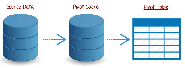
88. What exactly is a pivot cache?

Ans: 

A pivot cache is an internal data storage mechanism used by Excel to efficiently manage and handle the data source for a pivot table or pivot chart. It serves as an intermediary between the actual source data and the pivot table/chart. The pivot cache enhances the performance of pivot tables by optimizing data retrieval and manipulation, especially when dealing with large datasets.

89. Is it possible to create a Pivot Table from many tables?

Ans: 

• Navigate to the “Insert” tab and choose “PivotTable.”
• Select “Use an external data source” in the Create PivotTable dialog box and then click “Choose Connections.”
• Click “Add” in the Existing Connections dialog box to add your tables as connections.

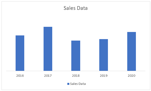
90. Explain a column chart.

Ans: 

A column chart is a type of graph used to visually represent data using vertical rectangular bars. Each bar in the column chart corresponds to a specific category or data point, and the height or length of the bar reflects the value of the data it represents. Column charts are effective for comparing values across different categories and showing trends or patterns within the data.

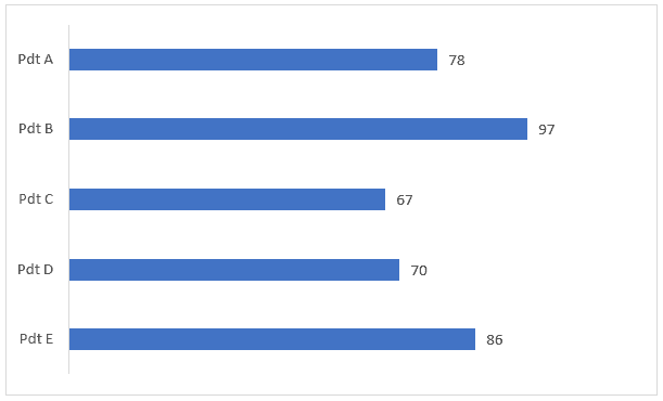
91. Describe a bar chart.

Ans: 

A bar chart is a visual depiction of data that uses horizontal bars to show information. Bar charts, like column charts, are useful for comparing values between categories or data points. The bars are arranged horizontally as opposed to vertically in a bar chart.

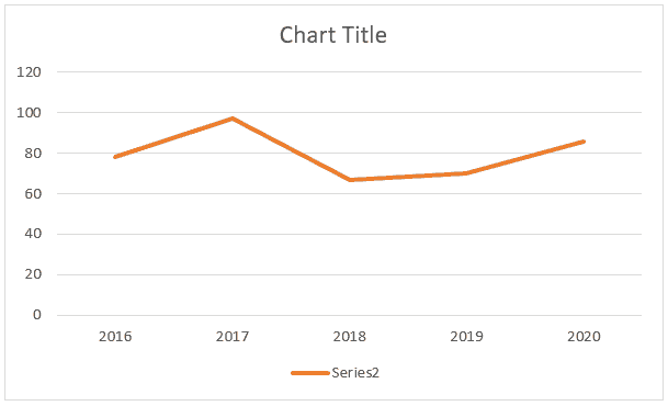
92. Describe a line chart.

Ans: 

A line chart is a particular form of graph used to show data trends and changes over an ongoing period of time. It creates a continuous line that depicts the evolution of values by connecting data points with straight lines. Line charts are excellent for depicting trends across time, contrasting numerous data series, and emphasizing connections between variables because they are particularly good at displaying patterns, trends, and oscillations in data.

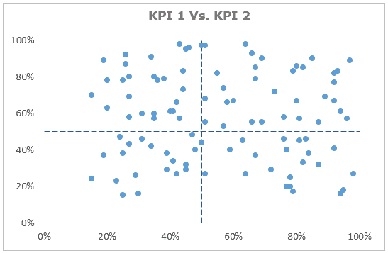
93. Describe the Scatter chart.

Ans: 

 A scatter chart, often called a scatter plot or scattergram, is a kind of graph that shows the relationship between two variables. Scatter charts emphasize individual data points and their distribution throughout the chart as opposed to line charts or bar charts, which highlight patterns or categories. Finding patterns, relationships, and outliers in data sets may be done very well with scatter plots.

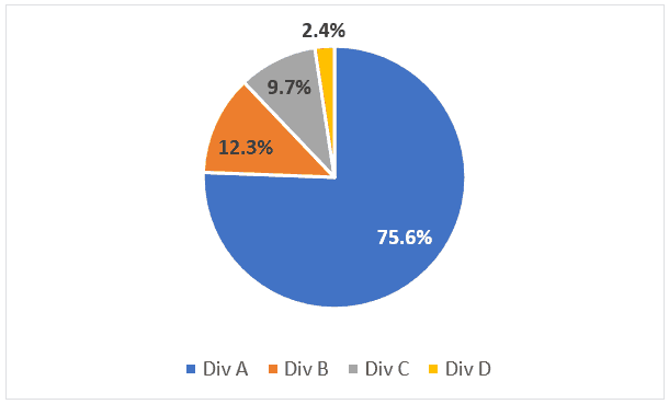
94. Do Pie charts work well? Does it belong in reports or the dashboard?

Ans: 

When displaying the proportionate distribution of several categories or components of a whole, pie charts may be a useful tool for data representation. The context and the number of categories involved can, however, affect how successful they are. Pie charts are effective when there are a limited number of categories and the variations between the categories are clear and distinguishable from one another by their sizes.

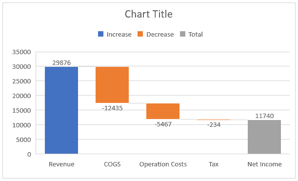
95. What is a Waterfall chart? When would you use it?

Ans: 

A Waterfall chart, also known as a bridge chart, is a specialized type of graph used to visualize incremental changes in a set of values over a series of categories. It’s particularly effective for showing how a starting value evolves through various positive and negative adjustments to reach a final value. Waterfall charts are commonly used in financial analysis, project management, and performance evaluation to illustrate the components contributing to a change in total.

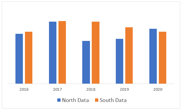
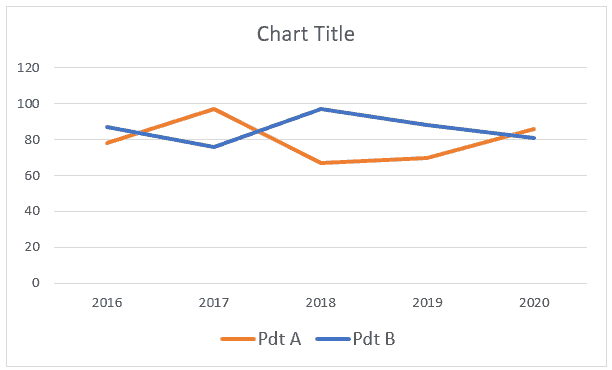
96. What are Combination charts?

Ans: 

Combination charts, commonly referred to as combo charts, are a form of Excel graph that let you present many sorts of data using various chart styles all inside the same chart. You may efficiently view and compare several sets of data that may have various scales, units, or features by combining two or more chart styles.

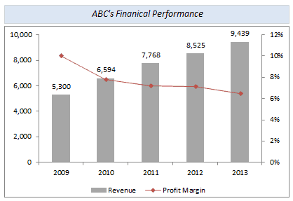
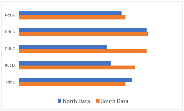
97. What is a secondary axis in a chart?

Ans: 

A secondary axis in a chart is an additional vertical (y) or horizontal (x) axis that is added to a chart to accommodate data series with different scales or units. It allows you to visually represent two or more sets of data that might have vastly different ranges or measurement units on the same chart. The secondary axis provides context and clarity when plotting data with significant variations in values.

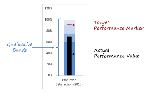
98. What is a Bullet chart? When should we use it?

Ans: 

A bullet chart is a specialized type of chart designed to display and compare a single metric against a target, as well as provide additional context in the form of qualitative ranges. Bullet charts are particularly effective for presenting performance data in a concise and informative manner.

99. How do I replace a value in Excel with another?

Ans: 

• To find the first occurrence of the value you wish to change, click “Find Next.”
• To find the following instance and replace the current one, click “Replace.”
• Replace all occurrences inside the chosen range by clicking “Replace All.”

100. How can you sort data in Excel?

Ans: 

To arrange data in a certain order depending on the values in one or more columns, you may sort it in Excel. Data organization by sorting facilitates information analysis, comparison, and discovery. Excel provides a variety of sorting choices, including ascending and descending order, sorting by several columns, and sorting by a single column.