Last updated on 23rd Apr 2025| 9227
- Introduction to Time Complexity
- Big O Notation: The Foundation of Time Complexity
- Common Time Complexities in Algorithms
- Best, Worst, and Average Case Analysis
- Space Complexity vs Time Complexity
- Analyzing Algorithm Performance with Examples
- Optimizing Algorithms for Better Efficiency
- Conclusion
Efficiency is key in determining an algorithm’s performance in computer science and programming, mainly as input data grows. Time complexity, which gauges how an algorithm’s execution time varies concerning input size, is crucial in evaluating its efficiency. Developers may assess their code’s scalability and ensure it functions properly, even with enormous datasets, by having a solid understanding of temporal complexity. Big O notation, which gives an upper bound on the rate at which the algorithm’s running time grows, is commonly used to define time complexity. For instance, an algorithm with a time complexity of O(n) means its running time increases linearly with the input size, while O(n^2) indicates that the time grows quadratically. By analyzing time complexity, developers can predict how their algorithms will behave as the input size grows and identify potential bottlenecks. Developers must understand Data Science Course Training time complexity because it allows them to write more efficient code, optimize performance, and make informed decisions about which Optimizing Algorithms to use for specific tasks. By the end of this post, you’ll better understand how to evaluate and improve the efficiency of your algorithms, ensuring your programs run smoothly, even as they scale.
Introduction to Time Complexity
Time complexity is a crucial metric in computer science that shows how an algorithm’s runtime develops as the size of its input increases. Because it enables developers to determine if an algorithm will scale well as input sizes grow without testing it on every potential input, this statistic is crucial. Hlookup in Excel of data frequently increases rapidly in real-world situations, which can have a big effect on how well a system or application performs. For example, if the dataset grows in size, an inefficient approach may result in longer processing times, which could cause the system to lag or even crash. Time complexity provides a way to predict how an algorithm will perform as the data size increases, helping developers identify potential performance bottlenecks before they arise. By understanding time complexity, developers can make more informed decisions when choosing or designing algorithms for specific tasks. This ensures that the software remains efficient and responsive, even as the amount of data scales, and helps avoid issues related to performance degradation as systems grow. Time complexity is key to writing software that performs well under various conditions, especially in data-intensive applications.
Become a Data Science expert by enrolling in this Data Science Online Course today.
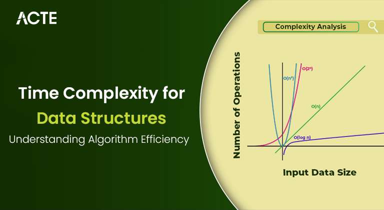
Big O Notation: The Foundation of Time Complexity
Big O notation is the mathematical framework used to express time complexity. It describes the upper bound of an algorithm’s running time in the worst-case scenario, helping us understand its scalability. Big O notation abstracts away constant factors and lower-order terms, focusing only on the Autoencoders in Deep Learning factors that affect performance as the input size grows. Here are a few examples of Big O notations and what they mean:
- O(1) Constant time complexity: The algorithm’s running time remains the same regardless of the input data size. For example, accessing an element in an array by its index is an O(1) operation.
- O(n): Linear time complexity: The algorithm’s running time grows linearly with the input size. A typical example is iterating over a list of n elements, where n is the number of elements in the list.
- O(n^2): Quadratic time complexity: This happens when the algorithm involves nested loops over the input data. A typical example is a naive sorting algorithm like Bubble Sort, where the time increases quadratically as the input grows.
Common Time Complexities in Algorithms
In this section, we will discuss the most common time complexities you’ll encounter in algorithm design:
- O(1) – Constant Time As mentioned earlier, O(1) means the algorithm takes the same time to run, regardless of the input size. Examples include accessing an element in a hash table or performing simple arithmetic operations.
- O(log n) – Logarithmic Time An algorithm is said to run in logarithmic time if Compare Two Columns in Excel time complexity grows logarithmically as the input size increases. Binary search is a classic example, where each step halves the input size.
- O(n) – Linear Time A linear-time algorithm processes each element of the input data once. For example, searching through an unsorted list of n elements is an O(n) operation.
- O(n log n) – Linearithmic Time: This complexity occurs in algorithms that break the problem into smaller parts and solve each recursively. Merge Sort and Quick Sort are algorithms running in O(n log n) time.
- O(n^2) – Quadratic Time: Quadratic time complexity arises when an algorithm performs a nested iteration over the input data. The Bubble Sort algorithm is a classic example.
- O(2^n) – Exponential Time: Exponential time complexity arises when the problem space grows exponentially with the input size. This is common in brute-force algorithms, like solving the traveling salesperson problem.
- O(n!) – Factorial Time: Factorial time complexity appears in Optimizing Algorithms that generate all possible permutations of an input. A brute-force approach to solving the N-Queens problem is an example.
- Best Case: This is the scenario where the algorithm performs the fewest operations. For example, the best case in Bubble Sort is when the list is sorted, and the algorithm goes through it once without swaps.
- Worst Case: The worst-case time complexity represents the maximum number of operations the algorithm will perform. Checkbox in Excel typically the most critical metric in time complexity analysis because it gives us an upper bound on performance. For example, the worst-case time complexity in Quick Sort is O(n^2) when the pivot is poorly chosen.
- Average Case: Given a random input, the average case represents the expected time complexity for an algorithm. It’s often calculated by assuming that all inputs are equally likely. For instance, the average case for Quick Sort is O(n log n), which is generally much faster than the worst case.
- Linear Search (O(n)): A linear search algorithm checks each element of an array to find a match. Since it needs to check each element in the worst case, its time complexity is O(n). As the array size increases, the Data Scientist Salary in India time grows linearly.
- Binary Search (O(log n)): Binary search is much more efficient than linear, especially with large data sets. It divides the data in half at each step, exponentially reducing the problem size. This leads to O(log n) time complexity, making it much faster than linear search for large datasets.
- Merge Sort (O(n log n)): Merge Sort is a divide-and-conquer algorithm that splits the array into smaller chunks, sorts them, and then merges them back together. This results in an O(n log n) time complexity, which is more efficient than Analyzing Algorithm like Bubble Sort.
- Use Efficient Algorithms: When possible, choose algorithms with better time complexities. For example, I prefer Quick Sort or Merge Sort (O(n log n)) over Bubble Sort (O(n^2)).
- Avoid Redundant Calculations: Cache results where applicable. For example, dynamic programming can help avoid recalculating values in recursive algorithms.
- Reduce Nested Loops: Nested loops often lead to higher Pandas vs Numpy . Consider restructuring the algorithm to reduce the number of nested loops or use more efficient data structures like hash tables to optimize lookups.
- Divide and Conquer: Breaking down problems into smaller subproblems and solving them independently can often lead to significant time savings. Divide and conquer algorithms, like Merge Sort and Quicksort, are good examples of this approach.
Advance your Data Science career by joining this Data Science Online Course now.
Best, Worst, and Average Case Analysis
Time complexity is often analyzed in terms of three cases:

Space Complexity vs Time Complexity
While time complexity is critical in analyzing an algorithm, it’s not the only one. Space complexity measures how much memory an algorithm needs relative to the input size. It’s essential to balance both time and space complexity. For example, an algorithm with O(n) time complexity but O(n^2) space complexity may not be feasible in practice due to memory limitations. Similarly, Data Science Course Training with optimal space complexity but suboptimal time complexity may be useless if it takes too long to execute. In some cases, you may need to optimize both aspects and understanding the complexity of time and space allows you to make more informed decisions.
Learn the fundamentals of Data Science with this Data Science Online Course .
Analyzing Algorithm Performance with Examples
Let’s look at a couple of Optimizing Algorithms and analyze their performance in terms of time complexity.
Are you getting ready for your Data Science interview? Check out our blog on Data Science Interview Questions and Answers!
Optimizing Algorithms for Better Efficiency
Conclusion
Understanding time complexity is crucial for every software developer or computer scientist. Data Science Course Training helps you evaluate and optimize algorithms, ensuring that your software performs well even as the size of the input grows. Time complexity provides a framework for analyzing how Analyzing Algorithm scale, and Big O notation is the standard tool for expressing this analysis. You can write more efficient, scalable, and maintainable code by becoming familiar with the different types of time complexities, understanding best, worst, and average case scenarios, and learning how to optimize algorithms. Whether working with small datasets or building large systems, time complexity will always be a fundamental factor when choosing the correct algorithm. Efficient algorithms are the backbone of successful software applications, and mastering the art of time complexity analysis is a key skill for any developer.