
Last updated on 21st Apr 2025| 10066
- What Does Excel’s HLOOKUP Mean?
- Excel Formula Format for HLOOKUP
- How Is HLOOKUP Used in Excel?
- HLOOKUP and VLOOKUP Differences
- Using HLOOKUP Across Worksheets
- HLOOKUP Approximate Match
- Conclusion
Excel offers several powerful functions to help users analyze and manage data effectively. One of the most useful functions for looking up data in a horizontal range is the HLOOKUP function. This function enables users to search for a specific value in the top row of a table and return a corresponding value from a specified row below it. The formula for HLOOKUP is structured as: =HLOOKUP(lookup_value, table_array, row_index_num, [range_lookup]). Here, lookup_value is the value you’re searching for, table_array is the range of data, row_index_num is the row number from which to return the value, and range_lookup is an optional argument to specify whether you want an exact or approximate match an essential Excel concept often covered in Data Science Training. HLOOKUP is particularly useful for tables organized horizontally. Unlike VLOOKUP, which searches data vertically in columns, HLOOKUP searches horizontally across rows, making it ideal for certain data layouts. Understanding the differences between these two functions can help improve your data analysis efficiency.
To Explore Data Science in Depth, Check Out Our Comprehensive Data Science Course Training To Gain Insights From Our Experts!
What Does Excel’s HLOOKUP Mean?
The Excel HLOOKUP function stands for “Horizontal Lookup” and allows users to search for a value in the top row of a table or range and return a corresponding value from a row beneath it. This function is particularly useful when working with large data tables where information is organized horizontally (across rows) rather than vertically (down columns), a concept that ties into the fundamentals of What is Data. HLOOKUP enables users to easily retrieve data from horizontal layouts, making it an essential tool for certain types of data analysis. Key points to note: HLOOKUP searches for a specified value in the top row (or another defined row) of a table, and returns the value from a row below it.
It functions similarly to VLOOKUP, which searches for values vertically within a column, but HLOOKUP is designed for horizontal data arrangement. For example, imagine a data table with the months of the year listed in the top row and corresponding sales figures in the row directly below. HLOOKUP can be used to search for a specific month and return the sales value for that month, providing an efficient way to access data within horizontally structured tables.
Excel Formula Format for HLOOKUP
The syntax of the HLOOKUP function in Excel is as follows: HLOOKUP(lookup_value, table_array, row_index_num, [range_lookup])
- lookup_value: The value you want to search for in the top row of the table or range.
- table_array: The range of cells that contains the data. The first row of this range is where HLOOKUP will search for the lookup_value.
- row_index_num: The row number in the table_array from which the value will be returned. The row number is counted starting from the first row in the table_array.
- [range_lookup]: An optional argument nt. It determines whether to find an exact match (FALSE) or an approximate match (TRUE or omitted by default), a detail often highlighted in What Is Data Processing.
- Exact or Approximate Match: When using the range_lookup argument, setting it to FALSE ensures that HLOOKUP finds an exact match. If set to TRUE (or omitted, as it is TRUE by default), HLOOKUP will return the closest match to the lookup_value, which may not be an exact match, but the nearest smaller value.
- Row Index Number Limitations: The row_index_num should be a positive integer that corresponds to a row number within the table_array. If the row number exceeds the number of rows in the table, HLOOKUP will return an error. Ensure that the row number provided is within the range of the table.
- Lookup Value Placement: The lookup_value must be located in the first row of the table_array. If the value is not in the top row, HLOOKUP won’t function correctly. The function specifically searches only in the top row for the lookup value.
- Column Alignment: HLOOKUP assumes that the values in the rows are aligned horizontally across columns. If your data is structured differently, HLOOKUP might not yield the desired results. Make sure the data is arranged in rows, with each value aligned under a column heading.
- If you have a data table with months in the top row and sales figures in the row beneath, HLOOKUP can help find the sales for a specific month.
- Example: To find the sales for March, use the formula: =HLOOKUP(“March”, A1:E2, 2, FALSE)
- This returns the value 1200, the sales figure under “March.”
- Instead of hardcoding a lookup value (e.g., “March”), you can reference a cell that contains the month.
- Example: If cell A4 contains “April,” the formula would be: =HLOOKUP(A4, A1:E2, 2, FALSE)
- This way, the formula dynamically updates based on the month entered in A4, returning the corresponding sales data a practical application often taught in Data Science Training.
- HLOOKUP can be used to search for a value across multiple datasets arranged horizontally.
- Example: If you have separate datasets for different regions, such as sales data for the North, South, East, and West regions in separate rows, HLOOKUP can quickly retrieve the value for any specific region based on the lookup value. =HLOOKUP(“North”, A1:E5, 3, FALSE)
- This searches for “North” in the top row and returns the corresponding value from the third row, making it easier to compare data across various categories or regions.
- Default Setting for Approximate Match: By default, the range_lookup argument in HLOOKUP is set to TRUE, allowing for approximate matches rather than exact matches. This is useful when you want to find the closest match to the lookup_value.
- Finding the Nearest Match: When range_lookup is set to TRUE, Excel will search for the nearest value that is less than or equal to the lookup_value. It will return the corresponding value from the row below.
- Data Must Be Sorted: For the function to work properly when range_lookup is TRUE, the data in the top row must be sorted in ascending order. If the data is not sorted, the results may be incorrect, a precision that mirrors the importance of data structure in Covariance vs Correlation.
- Example of Use: In a sales commission table, if the lookup value is $7,000, you would use the formula: =HLOOKUP(7000, A1:E2, 2, TRUE) This formula will return 15% because $5,000 is the closest value that is less than $7,000.
- Approximate Match in Real-World Scenarios: This setting is ideal when you’re working with ranges, such as tax brackets or commission rates, where exact matches aren’t always available, and the nearest match is acceptable.
To Earn Your Data Science Certification, Gain Insights From Leading Data Science Experts And Advance Your Career With ACTE’s Data Science Course Training Today!
How Is HLOOKUP Used in Excel?
Finding Sales Data for a Specific Month
Dynamic Lookup with Cell Reference
Lookup Across Different Datasets

HLOOKUP and VLOOKUP Differences
Both HLOOKUP and VLOOKUP are Excel functions used for searching data within a table, but they differ in the way the data is organized. HLOOKUP (Horizontal Lookup) searches for a lookup_value in the top row of a table and returns a value from a specified row beneath it. This function is useful when the data is arranged horizontally, with values spread across rows. On the other hand, VLOOKUP (Vertical Lookup) searches for the lookup_value in the first column of a table and returns a value from a column to the right, a method commonly introduced in What is Data Collection. This is typically used when the data is organized vertically, with values placed in columns. For example, consider a table for VLOOKUP with product IDs in the first row and corresponding products listed beneath them. To find the product associated with a particular ID (e.g., 102), you would use VLOOKUP. However, if the data is structured horizontally such as months listed across the top row with sales figures below HLOOKUP would be the more appropriate function.
Looking to Master Data Science? Discover the Data Science Masters Course Available at ACTE Now!
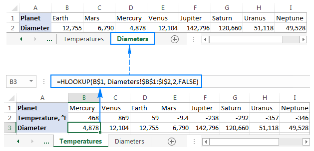
Using HLOOKUP Across Worksheets
One of HLOOKUP’s strengths is its ability to reference data on another worksheet within the same work. This is particularly useful when your data spans multiple sheets and you must perform lookups across them. To reference another worksheet in your HLOOKUP formula, include the sheet name before the range, separated by an exclamation mark (!). If your lookup table is in a worksheet called “SalesData,” the formula would look like this: =HLOOKUP(“January”, SalesData!A1:F2, 2, FALSE) This formula searches for “January” in the top row of the SalesData worksheet and returns the value from the second row of that sheet, showcasing skills relevant to Highest Paying Jobs in India. Using HLOOKUP Across Multiple Workbooks If the data is in another workbook, you can also use HLOOKUP with an external reference as long as the external workbook is open.
=HLOOKUP(“January”, ‘[SalesReport.xlsx]Sheet1’!A1:F2, 2, FALSE)
In this case, SalesReport.xlsx refers to the external workbook containing the data, and Sheet1 is the specific worksheet within that file. When using HLOOKUP across workbooks, you must reference both the workbook and sheet names correctly to retrieve the desired data, especially when pulling values from horizontally organized tables in another file.
HLOOKUP Approximate Match
Go Through These Data Science Interview Questions & Answer to Excel in Your Upcoming Interview.
Conclusion
The HLOOKUP function in Excel is a powerful tool for performing horizontal lookups, allowing users to find specific information in tables where data is organized in rows instead of columns. Understanding the formula structure, how to use it for dynamic lookups, and the key differences between HLOOKUP and VLOOKUP can help users fully utilize this function’s capabilities. HLOOKUP simplifies the process of retrieving values, whether you’re working with data from a single worksheet or multiple sheets, a function commonly explored in Data Science Training. It is particularly useful for tables where the lookup values are located in the top row, and the results are pulled from subsequent rows. Additionally, HLOOKUP becomes even more valuable when leveraging approximate matches, allowing for flexibility in data retrieval. Mastering HLOOKUP can significantly enhance your ability to analyze, manipulate, and report data effectively in Excel. As an essential part of the Excel toolkit, HLOOKUP improves both efficiency and accuracy in handling horizontally structured data, making it a must-have function for any data analyst.