What is Dimensionality Reduction? : ( A Complete Guide with Best Practices )

Last updated on 25th Dec 2021, Blog, General

(5.0) | 19897 Ratings 2001

Share:

Dimensionality reduction refers to techniques for reducing the number of input variables in training data. When dealing with high dimensional data, it is often useful to reduce the dimensionality by projecting the data to a lower dimensional subspace which captures the “essence” of the data.

• What is Dimensionality Reduction?
• The Curse of Dimensionality
• Benefits of applying Dimensionality Reduction
• Disadvantages of dimensionality Reduction
• Approaches of Dimension Reduction
• Feature Extraction
• Common techniques of Dimensionality Reduction
• The significance of Dimensionality Reduction
• Dimensionality Reduction Example
• Conclusion

What is Dimensionality Reduction?

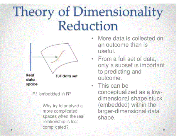
• The number of input features, variables, or columns present in a given dataset is known as dimensionality, and the process of reducing these features is called dimensionality reduction.


• The dataset contains a large number of input features in various cases, which further complicates the predictive modelling task. Because training datasets with a large number of features are very difficult to visualise or predict, for such cases, dimensionality reduction techniques need to be used.


• Dimensional reduction techniques can be defined as, “It is a method of converting a dataset of higher dimensions to a dataset of lower dimensions which ensures that it provides uniform information.” These techniques are widely used in machine learning to obtain a better fit predictive model while solving classification and regression problems.


• It is commonly used in fields that deal with high-dimensional data, such as speech recognition, signal processing, bioinformatics, etc. It can also be used for data visualisation, noise reduction, cluster analysis, etc.

The Curse of Dimensionality:

Handling high-dimensional data is very difficult in practice, which is commonly known as the curse of dimensionality. Any machine learning algorithm and model becomes more complex if the dimensionality of the input dataset increases. As the number of features increases, the number of samples also increases proportionally, and the probability of overfitting also increases. If a machine learning model is trained on high-dimensional data, it tends to overfit and result in poor performance.Therefore, there is often a need to reduce the number of features, which can be done with dimensionality reduction.

Benefits of applying Dimensionality Reduction:

Some of the benefits of applying dimensionality reduction technique to the given dataset are mentioned below:

• By reducing the dimensions of the features, the space required to store the dataset is also reduced.
• Fewer dimensions of the features require less computation training time.
• The reduced dimensions of the dataset’s features help to visualise the data quickly.
• It removes unnecessary features (if present) while taking care of multiplexing.

Disadvantages of dimensionality Reduction:

There are also some disadvantages of implementing dimensionality reduction, which are mentioned below:

• Some data may be lost due to dimensionality reduction.
• In PCA dimensionality reduction techniques, sometimes the principal components required to be considered are unknown.

Approaches of Dimension Reduction:

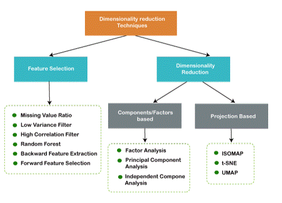
Feature selection is the process of selecting a subset of relevant features and discarding irrelevant features present in the dataset to build a model of high accuracy. In other words, it is a way of selecting the optimal features from the input dataset.

Three methods are used for feature selection:

1. Filter Methods

In this method, the dataset is filtered, and a subset containing only relevant features is taken. Some common techniques of the filter method are:

• Co – relationship
• Chi-square test
• anova
• information gain, etc.



2. Wrapper Methods

The wrapper method has the same goal as the filter method, but requires a machine learning model to evaluate. In this method, some features are fed to the ML model, and performance is evaluated. The performance decides whether to add or remove those features to increase the accuracy of the model. This method is more accurate than the filtering method but is more complicated to work with. Some common techniques of wrapper methods are:

• further selection
• backward selection
• bi-directional elimination



3. Embedded Methods: Embedded methods examine different training iterations of the machine learning model and evaluate the importance of each feature. Some common techniques of Embedded Methods are:

• Lasso
• elastic mesh
• Ridge regression, etc.

Feature Extraction:

Feature extraction is the process of converting a space of many dimensions into a space of lesser dimensions. This approach is useful when we want to have complete information but use less resources while processing the information:

Some common feature extraction techniques are:

• principal component analysis
• linear discriminant analysis
• Kernel PCA
• quadratic discriminant analysis

Common techniques of Dimensionality Reduction:

Principal Component Analysis (PCA)

Principal component analysis is a statistical procedure that converts an observation of correlated features into a set of linearly correlated features with the help of orthogonal transformations. These newly transformed characteristics are called principal components. It is a popular tool used for exploratory data analysis and predictive modelling.




Backward feature elimination

The backward feature elimination technique is mainly used when developing linear regression or logistic regression models. The following steps are followed in this technique in dimensionality reduction or feature selection: In this technique, all n variables of the given dataset are first taken to train the model.




The performance of the model is checked.

Now we will remove one feature each time and train the model n times on n-1 features, and calculate the performance of the model. We’ll examine the variable that caused the smallest or no change in the model’s performance, and then we’ll discard that variable or features; After that, we’ll be left with n-1 features.




Repeat the whole process until no feature drops.

In this technique, by selecting the optimal performance of the model and the maximum tolerable error rate, we can define the optimal number of features required for the machine learning algorithm.




Forward feature selection

Forward feature selection follows the inverse process of the backward elimination process. This means, in this technique, we do not eliminate the attribute; Instead, we will find the best features that can make the highest increase in the performance of the model. The following steps are followed in this technique: We start with just one feature, and gradually we’ll add each feature one at a time.




Missing value ratio

If a dataset has too many missing values, we discard those variables because they do not contain much useful information. To do this, we can set a threshold level, and if a variable is missing values ​​greater than that threshold, we will discard that variable. The higher the threshold value, the more efficient the reduction.




Low variance filter

Similar to the missing value ratio technique, a data column with few changes in the data contains less information. Therefore, we need to calculate the variance of each variable, and all data columns with variance less than a given threshold are discarded because low variance features will not affect the target variable.




Random forest

Random forest is a popular and very useful feature selection algorithm in machine learning. This algorithm has an in-built feature importance package, so we do not need to program it separately. In this technique, we need to generate a large set of trees against the target variable, and with the help of usage statistics of each feature, we need to find the subset of features. Random Forest algorithm takes only numeric variables, so we need to convert the input data into numeric data using hot encoding.




Factor analysis

Factor analysis is a technique in which each variable is placed within a group according to its correlation with other variables, meaning that variables within a group may have a high correlation with each other, but they may be correlated with variables in other groups. with low correlation. We can understand this with an example, like if we have two variables income and expenses. These two variables have a high correlation, meaning that people with higher incomes spend more, and vice versa. So, such variables are put in a group, and that group is known as a factor. The number of these factors will be reduced compared to the original dimension of the dataset.




Develop Your Skills with Dimensional Data Modeling Certification Training
Weekday / Weekend BatchesSee Batch Details

Auto-encoder

One of the popular methods of dimensionality reduction is the auto-encoder, which is a type of ANN or artificial neural network, and its main purpose is to copy the inputs to their outputs. In this, the input is compressed into a secret-space representation, and output is produced using this representation. It mainly consists of two parts:

Encoder: The function of the encoder is to compress the input so as to represent the hidden space.

Decoder: The function of the decoder is to reconstruct the output from the latent-space representation.

The significance of Dimensionality Reduction:

There are basically three reasons for dimensionality reduction:

• Visualization
• interpretability
• Time and space complexity



Let us understand this with an example:

• Imagine we have worked on a MNIST dataset which has 28×28 images and when we convert the images into features we get 784 features.
• If we try to think of each feature as a dimension, how can we think of 784 dimensions in our mind?
• We cannot imagine the scattering of points of 784 dimensions.
• This is the first reason why dimensionality reduction is important!
• Let’s say you are a data scientist and you have to explain your model to clients who don’t understand machine learning. How would you explain the working of 784 features or dimensions to them?

Dimensionality Reduction Example:

Here is an example of dimensionality reduction using the PCA method mentioned earlier. You want to classify a database full of emails into “not spam” and “spam”. To do this, you create a mathematical representation of each email as a bag-of-words vector. Each position in this binary vector corresponds to a word in the alphabet. For a single email, each entry in the bag-of-words vector is the number of times the corresponding word appears in the email (with a zero, meaning it doesn’t appear at all).




Now suppose you have constructed a bag-of-words from each email, which gives you a sample of bag-of-words vectors, X1…xm. However, the dimensions (words) of all your vectors are not useful for spam/not for spam classification. For example, words like “credit,” “bargain,” “offer,” and “sale” would be better candidates for spam classification than “sky,” “shoe,” or “fish.” This is where PCA comes in.




You should construct an M-by-M covariance matrix from your sample and calculate its eigenvectors and eigenvalues. Then sort the resulting numbers in descending order and choose the top eigenvalues ​​of p. By applying PCA to your vector samples, you project them onto the eigenvector corresponding to the top p eigenvalues. Your output data is now a projection of the original data onto p eigenvectors. Thus, the estimated data dimension has been reduced to p.




After computing the low-dimensional PCA projections of your bag-of-words vector, you can use the projection with various classification algorithms to classify emails instead of using the original email. Estimates are smaller than the original data, so things move faster.

Conclusion:

In machine learning, dimension refers to the number of features in a particular dataset. In simple words, dimensionality reduction refers to reducing the dimensions or features so that we can obtain a more explanatory model, and improve the performance of the model.




An intuitive example of dimensionality reduction can be discussed through a simple email classification problem, where we need to classify whether an email is spam or not. This can include a large number of features, such as whether the e-mail has a common title, the content of the e-mail, whether the email uses a template, etc. However, some of these features may overlap. In another situation, a classification problem that depends on both humidity and rainfall can be summed up in just one underlying feature, as both of the above are highly correlated. Therefore, we can reduce the number of features in such problems.




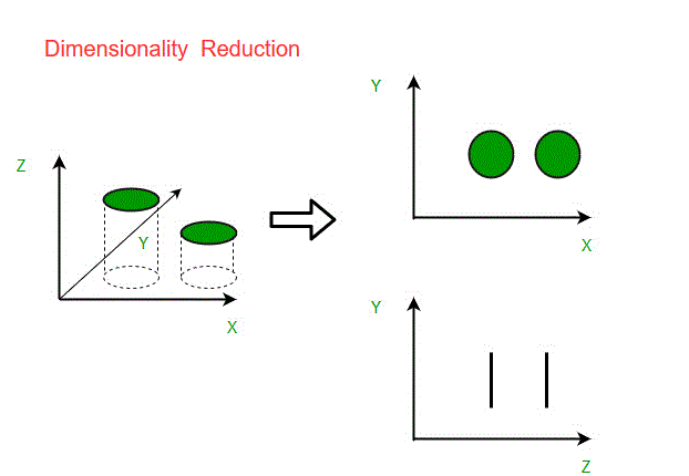
A 3-D classification problem can be difficult to visualise, whereas a 2-D one can be mapped to a simple 2-dimensional space and a 1-D problem to a simple line. The figure below illustrates this concept, where a 3-D feature space is split into two 1-D feature spaces, and subsequently, if found to be correlated, the number of features is further reduced. could.