
Last updated on 04th Jun 2025| 10807
- Understanding VLOOKUP Functionality
- Syntax and Parameters of VLOOKUP
- Using VLOOKUP for Exact Matches
- Using VLOOKUP for Approximate Matches
- Handling Errors in VLOOKUP
- Combining VLOOKUP with Other Functions
- VLOOKUP Across Multiple Worksheets
- Case Sensitivity and VLOOKUP
Understanding VLOOKUP Functionality
The VLOOKUP function in Excel is a powerful tool used to search for a value in the first column of a table range and return a corresponding value from another column in the same row. Short for “Vertical Lookup,” VLOOKUP is ideal for retrieving data from large datasets based on a specific reference value. The basic syntax of VLOOKUP is =VLOOKUP(lookup_value, table_array, col_index_num, [range_lookup]), where lookup_value is the value to search for, table_array is the range containing the data, col_index_num is the column number from which to return the result, and range_lookup determines whether the match should be exact (FALSE) or approximate (TRUE or omitted). Business Analyst Training shows that VLOOKUP is commonly used in tasks such as retrieving product details based on item codes, finding student grades from score lists, or mapping employee names to their IDs. For exact matches, the lookup column does not need to be sorted, but for approximate matches, it must be sorted in ascending order. While VLOOKUP is limited to searching only to the right of the lookup column, it remains highly useful when structured correctly. Advanced use cases often involve combining VLOOKUP with functions like IF, MATCH, and IFERROR to enhance flexibility and error handling. Despite the rise of more modern functions like XLOOKUP, VLOOKUP remains a fundamental and widely used function for data lookup in Excel.
Interested in Obtaining Your Business Analyst Certificate? View The Business Analyst Training Offered By ACTE Right Now!
Syntax and Parameters of VLOOKUP
The VLOOKUP function in Excel is used to search for a specific value in the first column of a table or range and return a corresponding value from another column in the same row. The syntax for VLOOKUP is: =VLOOKUP(lookup_value, table_array, col_index_num, [range_lookup]). The lookup_value is the value you want to find, which can be text, a number, or a cell reference. What is the ASAP Methodology explains that VLOOKUP searches for this value in the first column of the specified range. The table_array refers to the range of cells that contains the data. It must include the column where the lookup will happen and the column from which the result will be retrieved. The col_index_num is the column number in the table_array from which the matching value should be returned. The first column is numbered 1, the second is 2, and so on.
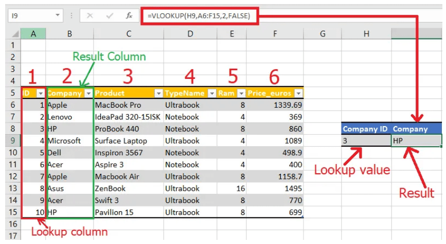
It’s important to provide the correct column index to avoid inaccurate results. The optional [range_lookup] argument determines the type of match: use FALSE for an exact match and TRUE (or omit it) for an approximate match. For approximate matches to work properly, the first column in the table_array must be sorted in ascending order. Understanding how these parameters work together allows users to effectively apply VLOOKUP in various data lookup and retrieval tasks within Excel spreadsheets.
Using VLOOKUP for Exact Matches
- Set the Range Lookup to FALSE: To perform an exact match, always set the fourth argument in the VLOOKUP function to FALSE. For example: =VLOOKUP(A2, B2:C10, 2, FALSE) ensures only exact matches are returned.
- Case Sensitivity Limitation: VLOOKUP is not case-sensitive, meaning it treats “Apple” and “apple” as the same. If case sensitivity is required, consider using other functions like INDEX and MATCH with EXACT.
- Avoid Sorted Data Requirement: How to Build a Successful Data Analyst Career highlights that, unlike approximate matches, exact-match VLOOKUP does not require the data to be sorted.
- Error Handling for Non-Matches: When an exact match isn’t found, VLOOKUP returns #N/A. Use IFERROR or ISNA to handle this gracefully: =IFERROR(VLOOKUP(A2, B2:C10, 2, FALSE), “Not Found”).
- Use with Data Validation: Exact-match VLOOKUP is ideal for validating data inputs. It can confirm whether a value exists in a reference list, improving data integrity in forms or spreadsheets.
- Supports Lookup on Text and Numbers: VLOOKUP with FALSE works with both numeric and text values, ensuring accurate results when matching IDs, codes, or names.
- Improves Data Accuracy: Exact match is crucial when working with critical data like pricing, inventory levels, or customer IDs, where incorrect matches could lead to significant errors.
- Set the Range Lookup to TRUE or Omit It: To perform an approximate match, set the fourth argument in the VLOOKUP function to TRUE or leave it blank. Example: =VLOOKUP(A2, B2:C10, 2, TRUE) returns the closest match less than or equal to the lookup value.
- Sort the Lookup Column in Ascending Order: For approximate matches to work correctly, the first column of the lookup range must be sorted in ascending order. Otherwise, VLOOKUP may return incorrect or unexpected results.
- Ideal for Grading or Tiered Pricing: Business Analyst Training teaches that approximate matches are useful for looking up values within a range, such as assigning letter grades, tax rates, or pricing tiers based on quantity or score.
- Returns the Closest Lower Match: VLOOKUP with TRUE finds the largest value that is less than or equal to the lookup value. If the lookup value is smaller than the lowest value in the column, it will return #N/A.
- Efficient for Large Datasets: Approximate match searches are generally faster, especially in large datasets, because they use binary search rather than scanning each row.
- No Duplicate Requirements: Unlike exact matches, the lookup column can contain repeated values; VLOOKUP will return the last appropriate match before exceeding the lookup value.
- Use with Numerical Ranges: Approximate match works best when mapping numeric inputs to output ranges, such as assigning discounts, scores, or performance categories.
- VLOOKUP with INDIRECT: Use INDIRECT to dynamically reference a range name or cell address for flexible lookups. Example: =VLOOKUP(A2, INDIRECT(B2), 2, FALSE).
- VLOOKUP with TEXT Functions: Clean or format data before lookup using functions like TRIM, UPPER, or TEXT to ensure accurate matches.
- VLOOKUP with IF: Use IF with VLOOKUP to return different results based on a condition. For example, =IF(VLOOKUP(A2, B2:C10, 2, FALSE)>100, “High”, “Low”) checks if the lookup value is above a threshold and returns custom text.
- VLOOKUP with ISERROR / IFERROR: Prevent errors when a lookup fails. =IFERROR(VLOOKUP(A2, B2:C10, 2, FALSE), “Not Found”) returns “Not Found” instead of an error if the value doesn’t exist in the lookup range.
- VLOOKUP with MATCH: Replace the hardcoded column index in VLOOKUP with MATCH for more dynamic formulas. Example: =VLOOKUP(A2, B2:E10, MATCH(“Sales”, B1:E1, 0), FALSE) adjusts the column index automatically.
- VLOOKUP with CONCATENATE / &: Books To Read For a Six Sigma Certification includes learning how to combine multiple columns into one lookup key. For example, =VLOOKUP(A2&B2, CHOOSE({1,2}, C2:C10&D2:D10, E2:E10), 2, FALSE) allows multi-criteria lookups.
- VLOOKUP with CHOOSE: Enables VLOOKUP to search from right to left. =VLOOKUP(A2, CHOOSE({1,2}, C2:C10, B2:B10), 2, FALSE) returns values from a column to the left of the lookup column.
To Earn Your Business Analyst Certification, Gain Insights From Leading Data Science Experts And Advance Your Career With ACTE’s Business Analyst Training Today!
Using VLOOKUP for Approximate Matches

Handling Errors in VLOOKUP
While VLOOKUP is a powerful function in Excel, it can sometimes return errors when it fails to find a match or encounters invalid inputs. One of the most common errors is #N/A, which appears when the lookup value does not exist in the first column of the table_array. This can occur due to misspelled text, incorrect formatting, or when the data is simply not present. To handle such cases gracefully, you can use the IFERROR function, which catches errors and allows you to display a custom message instead. What is SAP Certification explains that, for example, =IFERROR(VLOOKUP(A2, B2:C10, 2, FALSE), “Not Found”) will return “Not Found” instead of #N/A. Another approach is using ISNA in combination with IF, such as =IF(ISNA(VLOOKUP(…)), “Not Available”, VLOOKUP(…)), though IFERROR is simpler and more efficient in most cases. Errors can also result from incorrect column index numbers or improperly structured table arrays. It’s essential to ensure the lookup column is the first column in the range and that the col_index_num refers to a valid column within the table_array. Additionally, when using approximate matches, the first column must be sorted in ascending order; otherwise, VLOOKUP may return incorrect results or #N/A. Handling these potential errors proactively improves the reliability and readability of your formulas, leading to a smoother and more user-friendly Excel experience.
Want to Pursue a Business Intelligence Master’s Degree? Enroll For Business Intelligence Master Program Training Course Today!
Combining VLOOKUP with Other Functions
VLOOKUP Across Multiple Worksheets
VLOOKUP can be effectively used across multiple worksheets in Excel to retrieve data from different sources within the same workbook. This is particularly useful when data is organized by categories, departments, or time periods across separate sheets. To use VLOOKUP across worksheets, you need to reference the sheet name in the table_array argument. The general syntax remains the same: =VLOOKUP(lookup_value, SheetName!range, col_index_num, [range_lookup]). For example, =VLOOKUP(A2, ‘Sales 2024’!B2:D100, 2, FALSE) searches for the value in cell A2 on the ‘Sales 2024’ sheet within the specified range and returns the corresponding value from the second column. Which Certification is Right for You: Six Sigma or Lean Six advises making sure the sheet name is enclosed in single quotes if it contains spaces or special characters. The structure of the lookup table must remain consistent across worksheets for the formula to return accurate results. To make formulas easier to manage, you can also use named ranges that span across worksheets, especially when referring to the same data layout. When performing lookups across sheets, it’s important to check that all sheet references are correct and the data is up to date. Errors like #REF! can occur if a referenced sheet is renamed or deleted. Using VLOOKUP across multiple worksheets improves organization and enables centralized data analysis without duplicating information, making large workbooks more efficient and manageable.
Are You Preparing for Business Analyst Jobs? Check Out ACTE’s Business Analyst Interview Questions and Answers to Boost Your Preparation!
Case Sensitivity and VLOOKUP
By default, the VLOOKUP function in Excel is not case-sensitive, meaning it treats uppercase and lowercase letters as the same. For example, VLOOKUP will consider “APPLE” and “apple” to be identical values and return the first matching result regardless of letter casing. This can be a limitation in scenarios where case differentiation is crucial, such as product codes, passwords, or case-specific identifiers. To perform a case-sensitive lookup, VLOOKUP alone is insufficient. Instead, you need to combine other functions like INDEX, MATCH, and EXACT. Business Analyst Training covers the EXACT function, which compares two text values and returns TRUE only if they match exactly, including case. An example of a case-sensitive formula would be: =INDEX(return_range, MATCH(TRUE, EXACT(lookup_value, lookup_range), 0)). This array formula (entered using Ctrl+Shift+Enter in some Excel versions) allows you to find the position of an exact case-sensitive match and retrieve the corresponding value from another range using INDEX. It’s also essential to ensure consistent formatting of data, as unintentional differences in case can cause misinterpretations. While VLOOKUP is powerful for general lookups, for case-specific requirements, using alternative formulas with EXACT provides greater precision. Understanding VLOOKUP’s lack of case sensitivity helps avoid unexpected results and ensures the appropriate approach is chosen when working with case-sensitive data in Excel.