Last updated on 08th Aug 2025| 12178
- What is Time Series Data?
- Components of Time Series (Trend, Seasonality)
- Time Series Decomposition
- Moving Averages and Smoothing
- Autocorrelation and ACF/PACF
- ARIMA Model
- LSTM for Time Series Forecasting
- Evaluation Metrics for Time Series
- Stationarity and Differencing
- Case Studies in Finance and Weather
- Conclusion
What is Time Series Data?
Time series data consists of observations collected sequentially over time. Each data point is associated with a timestamp, and the order of the data is crucial. Common examples include stock prices, temperature recordings, electricity usage, and economic indicators. Machine Learning Training covers time series modeling techniques such as ARIMA, LSTM, and Prophet to analyze and forecast sequential data effectively. What distinguishes time series data from other types is its inherent temporal ordering: future values often depend on past values, making time a critical element. Time series analysis involves techniques to analyze historical data to extract meaningful statistics, detect patterns, and make forecasts. These methods are widely used across domains such as finance, weather forecasting, energy management, and retail.
Ready to Get Certified in Machine Learning? Explore the Program Now Machine Learning Online Training Offered By ACTE Right Now!
Components of Time Series
Understanding the internal structure of a time series is key for effective data analysis. A time series has four main components that together reveal its underlying behavior. These components can be modeled and interpreted using principles from Pattern Recognition and Machine Learning, which provide statistical and algorithmic tools to identify trends, seasonality, and noise. Such techniques enable systems to learn temporal patterns and make accurate predictions over time. The trend shows the long-term direction, indicating whether the series is rising or falling over a long time. Seasonality captures short-term cycles that repeat at regular intervals, like daily, monthly, or yearly patterns.
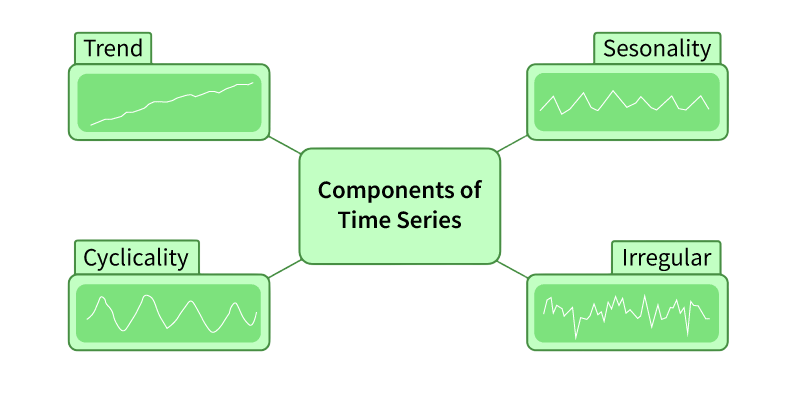
Cyclic patterns differ from seasonality because they show longer-term changes that do not have a set duration, often reflecting wider economic or environmental shifts. Additionally, irregular components, or ‘noise’, represent random changes that cannot be linked directly to trend, seasonality, or cyclic movements. Analysts can model these components either by adding them together or by multiplying them, based on the specific characteristics and behavior of the series.
Time Series Decomposition
Decomposition is a technique used to split a time series into its underlying components trend, seasonality, and residual (noise). This helps in better understanding the structure of the data and is often a precursor to forecasting. These analytical steps can be efficiently executed using cloud-based platforms like Overview of ML on AWS, which offers scalable tools such as Amazon SageMaker for building, training, and deploying models that learn from temporal patterns and adapt to evolving data streams.
There are two main types of decomposition:
- Additive Model: Y(t) = T(t) + S(t) + E(t)
- Multiplicative Model: Y(t) = T(t) × S(t) × E(t)
Python’s statsmodels library provides a seasonal_decompose function to perform this decomposition effectively.
To Explore Machine Learning in Depth, Check Out Our Comprehensive Machine Learning Online Training To Gain Insights From Our Experts!
Moving Averages and Smoothing
Smoothing techniques help reduce noise in a time series, making the trend and seasonal patterns more visible.
Types of Moving Averages:
- Simple Moving Average (SMA): Averages over a fixed number of past periods.
- Weighted Moving Average (WMA): Weights more recent values more heavily.
- Exponential Moving Average (EMA): Uses exponential weighting to emphasize recent data.
These techniques are especially useful for identifying long-term trends and preparing the data for modeling.

Autocorrelation and ACF/PACF
Autocorrelation measures how similar a time series is to its past versions. It helps reveal important patterns and dependencies. Researchers and data scientists use the Autocorrelation Function (ACF) and Partial Autocorrelation Function (PACF) as key tools to understand the time relationships in time series data. Machine Learning Training explains how ACF and PACF plots guide model selection for ARIMA and other time series forecasting techniques. By looking at how a series relates to its past values, these plots provide important information for deciding the right order of autoregressive (AR) and moving average (MA) components in ARIMA models. Modern statistical libraries like Python’s statsmodels have made this process easier. They offer built-in functions that let researchers efficiently create ACF and PACF plots, helping improve time series analysis.
ARIMA Model
ARIMA (AutoRegressive Integrated Moving Average) serves as a cornerstone in time series forecasting, providing a sophisticated approach to predictive modeling by integrating three key components, autoregression, integration, and moving average. This model excels at capturing complex temporal patterns by regressing a variable against its past values (AR), differencing raw observations to ensure stationarity (I), and modeling error as a linear combination of past error terms (MA). These forecasting techniques can be implemented using deep learning frameworks like Keras vs TensorFlow, where Keras offers a user-friendly API for rapid prototyping, and TensorFlow provides scalable infrastructure for production-grade time series models. Represented as ARIMA(p,d,q), where p, d, and q are carefully determined parameters, analysts must conduct meticulous analysis using techniques like ACF/PACF plots and stationarity tests. Data scientists can easily implement ARIMA in Python with libraries like statsmodels, allowing them to construct predictive models that forecast future trends with remarkable precision and reliability.
Looking to Master Machine Learning? Discover the Machine Learning Expert Masters Program Training Course Available at ACTE Now!
LSTM for Time Series Forecasting
Long Short-Term Memory (LSTM) networks are a special type of Recurrent Neural Networks (RNNs) designed to learn from sequences. They excel at capturing long-term dependencies, making them ideal for time series with complex patterns. These models are often built using Machine Learning Tools that provide scalable frameworks, intuitive APIs, and optimized workflows for training and deploying sequence-aware architectures.
Key Features:
- Handles non-linearities and interactions
- Remembers long-term dependencies
- Works well on multivariate time series
Evaluation Metrics for Time Series
Evaluating time series models involves specific metrics different from classification tasks:
- Mean Absolute Error (MAE): Average of absolute differences between actual and predicted values.
- Mean Squared Error (MSE): Average of squared differences, penalizes larger errors more heavily.
- Root Mean Squared Error (RMSE): Square root of MSE, expressed in the same units as the original data.
- Mean Absolute Percentage Error (MAPE): Percentage-based error, useful for interpretability across scales.
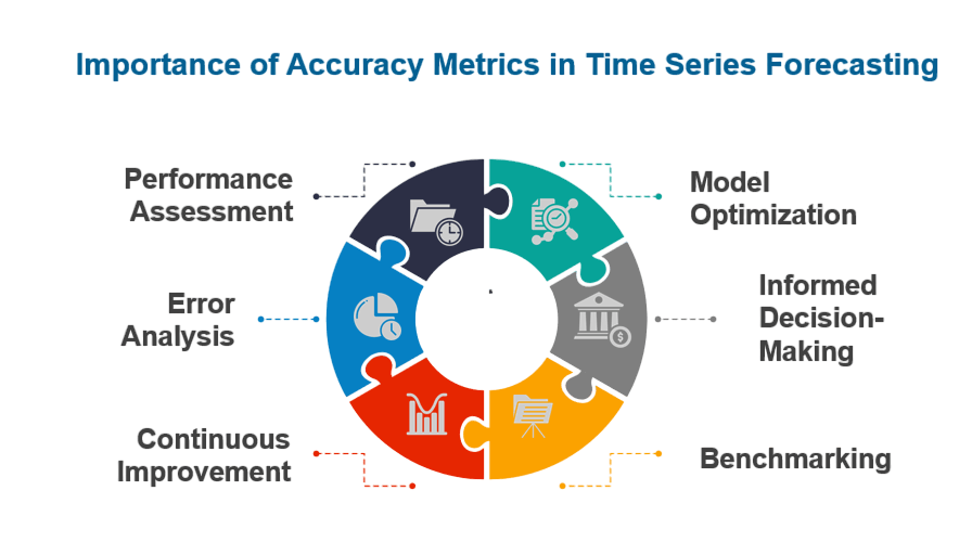
Choosing the right metric depends on the business context and sensitivity to large deviations.
Preparing for Machine Learning Job Interviews? Have a Look at Our Blog on Machine Learning Interview Questions and Answers To Ace Your Interview!
Stationarity and Differencing
A stationary time series has a constant mean and variance over time. Many models like ARIMA assume stationarity, making stationarity testing and transformation critical. These preprocessing steps are essential in domains like forecasting and anomaly detection, where roles such as Machine Learning Engineer Salary often reflect the complexity and impact of deploying robust time series models in production environments.
Testing Stationarity:
- Visual inspection: Check mean and variance consistency over time.
- Augmented Dickey-Fuller (ADF) test: Statistical test for detecting stationarity.
Making Data Stationary:
- Differencing: Subtracting a previous observation from the current to remove trends.
- Log transformation: Reduces variance and stabilizes fluctuations.
- Seasonal differencing: Removes repeating seasonal effects from the series.
Differencing is denoted by the d parameter in ARIMA models.
Case Studies
Finance (Stock Price Forecasting)
- Problem: Predicting short-term stock trends
- Model: ARIMA or LSTM
- Challenge: High noise, external factors
- Metric: RMSE or directional accuracy
- Outcome: ARIMA provides quick baselines; LSTM often outperforms with longer historical data.
Weather Forecasting
- Problem: Predicting temperature, rainfall, wind speed
- Model: SARIMA, LSTM, Prophet
- Challenge: Complex seasonality and cyclic behavior
- Metric: MAE, MAPE
- Outcome: SARIMA handles seasonality well; LSTM captures complex interactions.
Conclusion
Time series analysis is a powerful field that affects many industries. It helps organizations predict sales, manage energy needs, and make smart financial choices.By using various analytical methods, including traditional statistical models like ARIMA and SARIMA, as well as deep learning techniques like LSTM and tools like Prophet, professionals gain valuable insights. Machine Learning Training equips practitioners with the skills to choose and apply the right forecasting models based on data patterns and business needs. Effective time series analysis requires a clear process. This starts with data visualization and involves using decomposition and smoothing techniques to identify patterns. It also requires testing for data stationarity and choosing appropriate evaluation metrics for the specific area. Additionally, combining statistical and machine learning methods improves forecasting accuracy and offers detailed strategic insights. When done skillfully, time series analysis goes beyond simple calculations and provides actionable forecasts that significantly impact business, science, and technology.