Last updated on 08th Aug 2025| 12466
- Introduction to Gradient of a Function
- Role in Optimization
- Mathematical Definition
- Partial Derivatives and Multivariable Functions
- Gradient Descent Algorithm
- Variants of Gradient Descent
- Applications in Machine Learning
- Visualization of Gradients
- Gradient vs Directional Derivative
- Challenges in Gradient Computation
- Summary and Use Cases
Introduction to Gradients
Gradients are the cornerstone of optimization techniques used in machine learning and deep learning. They are vectors that point in the direction of the greatest rate of increase of a function and are essential in determining how to adjust parameters to minimize a loss function. Understanding gradients is fundamental for Machine Learning Training, especially in neural networks, where optimization plays a central role. This guide provides a comprehensive understanding of gradients, covering their mathematical foundations, implementation in gradient-based optimization methods, and relevance in real-world machine learning applications.
Ready to Get Certified in Machine Learning? Explore the Program Now Machine Learning Online Training Offered By ACTE Right Now!
Role in Optimization
Optimization in machine learning refers to the process of minimizing (or maximizing) a function to improve model performance.
Mathematical Definition
To understand the foundation, it’s useful to ask What Is Machine Learning. Mathematically, the gradient is a vector of partial derivatives:
- ∇f(x)=[∂f∂x1,∂f∂x2,…,∂f∂xn]\nabla f(\mathbf{x}) = \left[\frac{\partial f}{\partial x_1}, \frac{\partial f}{\partial x_2}, \ldots, \frac{\partial f}{\partial x_n}\right]
- x=[x1,x2,…,xn]\mathbf{x} = [x_1, x_2, \ldots, x_n].
Here, is a scalar-valued function of multiple variables, and each component of the gradient vector represents the rate of change of the function with respect to one of the variables. The gradient points in the direction of the steepest ascent of the function. For minimization tasks, optimization algorithms typically move in the opposite direction of the negative gradient.
To Explore Machine Learning in Depth, Check Out Our Comprehensive Machine Learning Online Training To Gain Insights From Our Experts!
Partial Derivatives and Multivariable Functions
Partial derivatives measure how a function changes as one of its input variables changes while keeping the others constant. They are building blocks for constructing gradients in multivariable functions. For a function f(x,y)f(x, y), the partial derivatives are:
- ∂f∂x,∂f∂y\frac{\partial f}{\partial x}, \quad \frac{\partial f}{\partial y}
These indicate how the function changes as x or y changes independently. The gradient combines these into a vector that can be used for optimization.

Gradient Descent Algorithm
Gradient Descent is a key optimization algorithm in machine learning. It provides a strong method for improving model parameters. Machine Learning Training enables effective loss reduction by updating parameters in the direction opposite to the gradient. The main update rule, θ = θ − η∇L(θ), clearly illustrates this process. Here, θ stands for the model parameters, η is the learning rate, and ∇L(θ) indicates the Gradient of a Function. This step-by-step method allows models to gradually reach better performance. Gradient Descent is essential for training complex machine learning systems in many different areas.
Variants of Gradient Descent
In machine learning optimization, gradient descent algorithms offer different ways to train models. Ensemble methods like Bagging vs Boosting offer different strategies for model improvement. Meanwhile, Batch Gradient Descent processes the entire dataset in one go, providing thorough but resource-heavy updates. Stochastic Gradient Descent (SGD) takes a different route by updating parameters based on individual samples, which improves efficiency. Mini-batch Gradient Descent finds a middle ground by using small groups of samples to balance resource use and model performance. Building on these basic ideas, optimizers like Adam, RMSprop, and Adagrad have come up, improving gradient descent methods to boost learning dynamics and speed up convergence in complex neural network designs.
Looking to Master Machine Learning? Discover the Machine Learning Expert Masters Program Training Course Available at ACTE Now!
Applications in Machine Learning
Gradients are indispensable in training:
- Neural Networks: Backpropagation uses gradients to update weights.
- Linear/Logistic Regression: Closed-form or iterative gradient updates.
- Support Vector Machines: Optimization using gradient-based solvers.
- Reinforcement Learning: Policy gradients for optimizing strategies.
They help models learn the patterns from data by continuously minimizing loss functions.
Visualization of Gradients
Visualizing gradients can provide intuitive understanding. Consider a contour plot of a function with gradient vectors drawn at various points. The vectors point perpendicular to the contours and indicate the direction of the steepest ascent. In 2D, gradient descent can be visualized as a ball rolling down a hill, with the slope at each point determined by the gradient.
- import numpy as np
- import matplotlib.pyplot as plt
- x, y = np.meshgrid(np.linspace(-2, 2, 20), np.linspace(-2, 2, 20))
- z = x**2 + y**2
- dz_dx = 2 * x
- dz_dy = 2 * y
- plt.contour(x, y, z, levels=20)
- plt.quiver(x, y, dz_dx, dz_dy)
- plt.title(‘Gradient Field for f(x, y) = x^2 + y^2’)
- plt.xlabel(‘x’)
- plt.ylabel(‘y’)
- plt.show()
Preparing for Machine Learning Job Interviews? Have a Look at Our Blog on Machine Learning Interview Questions and Answers To Ace Your Interview!
Gradient vs Directional Derivative
In mathematical analysis, Gradient vs Directional Derivatives are important for understanding rates of change. The directional derivative, shown as Duf(x) = ∇f(x) ⋅ u, measures how a function changes in any specific direction using a unit vector u. Tools like the Confusion Matrix in Machine Learning help mathematicians and scientists calculate how a function varies when moving in a certain direction. The directional derivative reaches its maximum value when the unit vector aligns perfectly with the gradient. This provides key insights into the function’s behavior and slope characteristics. By gradient vs directional derivative projecting the gradient onto the chosen direction, researchers can measure and understand the most significant rates of change in multidimensional spaces.
Challenges in Gradient Computation
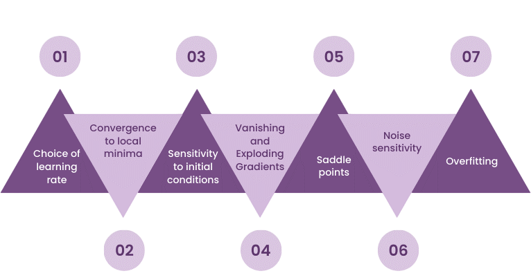
Machine Learning Algorithms are widely used across domains, but some practical issues in gradient computation include:
- Vanishing Gradients: Gradients become too small to affect updates. Common in deep or recurrent networks.
- Exploding Gradients: Large gradients cause unstable updates.
- Non-differentiable Functions: Require subgradient methods or approximations.
- Plateaus and Saddle Points: Flat regions with near-zero gradients slow learning.
Gradient computation techniques like gradient clipping, careful initialization, and using ReLU activations help mitigate these problems.
Numerical vs Symbolic Gradients
- Symbolic Differentiation: Uses calculus rules to derive expressions for gradients. Exact but may be complex.
- Numerical Differentiation: Approximates gradient using finite differences.
Summary and Use Cases
Gradients drive machine learning optimization by guiding model training. They show how parameters should change to reduce error. These mathematical tools provide important insights, allowing Machine Learning Training algorithms like gradient descent to improve model performance through careful parameter adjustments. Deep neural networks use the chain rule to spread error signals effectively, and some methods deal with problems like vanishing gradients. Gradients are crucial for training complex neural networks and fine-tuning parameters in areas like computer vision and natural language processing. Their ability to visualize and calculate the steepest increases in functions makes them vital tools for data scientists who want to create efficient, high-performance models that solve complex computational challenges with accuracy.