
Last updated on 13th Aug 2025| 12923
- Introduction to Decision Tree Algorithm
- Tree Structure and Terminology
- Splitting Criteria (Gini, Entropy)
- Overfitting and Pruning
- Decision Tree Algorithm in Classification and Regression
- Implementation in Python
- Visualizing Decision Trees
- Applications in Industry
- Ensemble Methods (Random Forest, Boosting)
- Hyperparameter Tuning
- Summary
Introduction to Decision Tree Algorithm
Decision Trees are one of the most intuitive and widely used machine learning algorithms. They are non-parametric models used for both classification and regression tasks. A decision tree learns rules from data features to predict target values by splitting the data into subsets based on feature value tests. These splits form a tree-like structure where each internal node represents a test on a feature, each branch represents the outcome of the test, and each leaf node represents a prediction an architecture thoroughly dissected in Machine Learning Training, where learners explore decision trees, entropy calculations, and recursive partitioning to build interpretable models. The simplicity and interpretability of decision trees make them a popular choice for both academic learning and real-world applications. Despite their simplicity, they form the basis for powerful ensemble methods like Random Forest and Gradient Boosted Trees.
Tree Structure and Terminology
To understand decision trees, one must explore their complex structure and specific terms. At the center of this framework is the root node, which represents the entire dataset and starts the first split. As the tree grows, internal nodes appear, testing and assessing features to divide the dataset. These branches link nodes, showing specific test results and guiding how the tree develops. To understand how this structure fits into broader modeling techniques, exploring Machine Learning Algorithms reveals essential methods like Decision Trees, Random Forests, SVMs, and Gradient Boosting each offering unique strengths for classification, regression, and pattern recognition across diverse datasets and problem domains. Leaf nodes, or terminal nodes, ultimately hold the final prediction or output. The tree’s depth is defined by the number of levels from the root to its deepest leaf. The processes of splitting and pruning allow for better data segmentation and improvement by dividing nodes and removing less meaningful branches. Grasping these basic elements offers clear insight into how decision tree algorithms work.
Ready to Get Certified in Machine Learning? Explore the Program Now Machine Learning Online Training Offered By ACTE Right Now!
Splitting Criteria (Gini, Entropy)
The core idea of a decision tree is to find the best attribute that splits the dataset into homogeneous subsets. The quality of a split is measured using metrics like: information gain, Gini impurity, and gain ratio. To reinforce this concept with hands-on experience, exploring Machine Learning Projects reveals beginner-friendly applications such as sales forecasting, wine quality prediction, and handwritten digit classification each designed to help learners apply decision tree logic, evaluate split criteria, and build interpretable models using real-world datasets.
Gini Impurity
It measures the frequency at which a randomly chosen element would be incorrectly classified. The formula is:
- Gini=1−∑i=1npi2Gini = 1 – \sum_{i=1}^{n} p_i^2
- IG=Entropy(parent)−∑j(njn×Entropy(j))IG = Entropy(parent) – \sum_{j} \left( \frac{n_j}{n} \times Entropy(j) \right)
where pip_i is the probability of an element being classified to a particular class.
Higher information gain or lower Gini impurity signifies a better split.
Overfitting and Pruning
One of the primary issues with decision trees is overfitting and pruning , where the tree becomes too complex and captures noise in the training data.
Solutions:
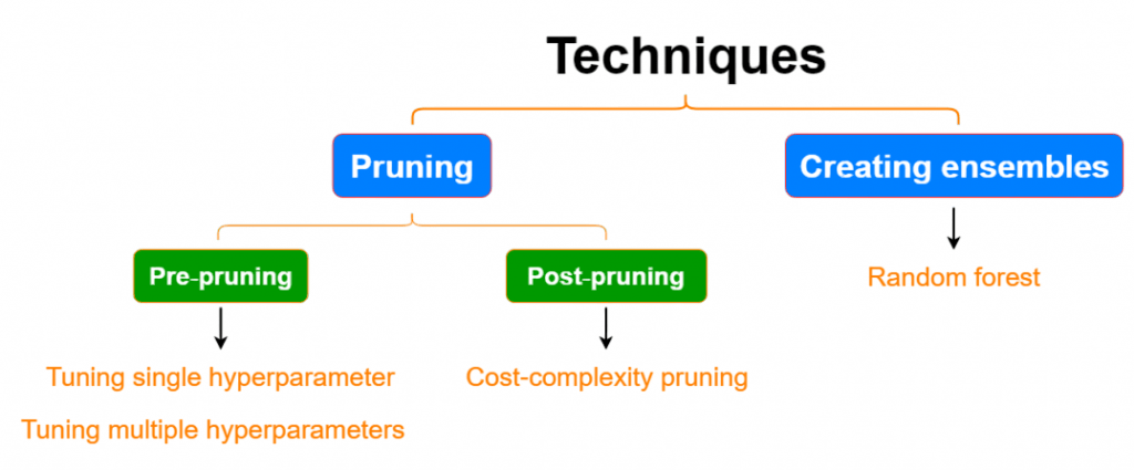
- Pre-Pruning (Early Stopping): Stop splitting if the node has fewer than a set number of instances or a maximum depth is reached.
- Post-Pruning: Grow the full tree and then remove branches that do not contribute significantly to prediction accuracy.
Pruning helps improve generalization by simplifying the tree structure.
To Explore Machine Learning in Depth, Check Out Our Comprehensive Machine Learning Online Training To Gain Insights From Our Experts!
Decision Tree Algorithm in Classification and Regression
Classification and regression trees are effective machine learning techniques that serve different purposes based on the type of target variable. Classification trees are made for categorical target variables a foundational concept in Machine Learning Training, where learners explore decision tree structures, splitting criteria, and classification algorithms to build accurate predictive models. Each leaf node represents a unique class label, allowing for accurate categorization. On the other hand, regression trees are used for continuous target variables. Here, leaf nodes predict the average value of outputs within that specific node. A key feature of regression trees is their splitting criteria, which usually use metrics like Mean Squared Error (MSE) instead of traditional classification metrics like Gini impurity or entropy. These tree-based models offer clear and understandable methods for predictive modeling. They help data scientists capture complex relationships in datasets while keeping computational efficiency.

Implementation in Python
Decision trees can be easily implemented using libraries like Scikit-learn. To complement these tree-based models with a foundational classification technique, exploring Logistic Regression reveals how the sigmoid function transforms linear outputs into probabilities enabling binary and multiclass predictions that are both interpretable and efficient, especially for linearly separable datasets and baseline modeling in machine learning workflows.
- from sklearn.datasets import load_iris
- from sklearn.tree import DecisionTreeClassifier
- from sklearn.model_selection import train_test_split
- from sklearn.metrics import accuracy_score
- # Load dataset
- iris = load_iris()
- X_train, X_test, y_train, y_test = train_test_split(iris.data, iris.target, test_size=0.3)
- # Create and train model
- clf = DecisionTreeClassifier(criterion=’gini’, max_depth=3)
- clf.fit(X_train, y_train)
- # Predict and evaluate
- y_pred = clf.predict(X_test)
- print(“Accuracy:”, accuracy_score(y_test, y_pred))
Looking to Master Machine Learning? Discover the Machine Learning Expert Masters Program Training Course Available at ACTE Now!
Visualizing Decision Trees
Visualizing Decision Trees helps in understanding how decisions are being made. To complement this interpretability with performance diagnostics, exploring Confusion Matrix in Machine Learning reveals how classification outcomes true positives, false positives, true negatives, and false negatives are organized into a matrix that helps quantify model accuracy, precision, recall, and error types, offering a clearer view of how well the decision tree is performing across different classes.
- from sklearn.tree import plot_tree
- import matplotlib.pyplot as plt
- plt.figure(figsize=(12, 8))
- plot_tree(clf, feature_names=iris.feature_names, class_names=iris.target_names, filled=True)
- plt.show()
- # Other visualizing decision trees tools include Graphviz and the export_graphviz() function for more detailed rendering
Applications in Industry
Decision trees are used in a variety of real-world applications:
- Finance: Credit scoring, risk management.
- Healthcare: Diagnosing diseases, treatment recommendations.
- Marketing: Customer segmentation, churn prediction.
- Manufacturing: Quality control, defect detection.
- Retail: Product recommendation, inventory management.
Their transparency and interpretability make them especially useful in regulated industries. To enhance these qualities with ensemble strategies, exploring Bagging vs Boosting in Machine Learning reveals how bagging reduces variance by training models independently on random subsets, while boosting reduces bias by sequentially correcting errors both improving model stability and offering explainable decision paths that align well with compliance-driven environments.
Preparing for Machine Learning Job Interviews? Have a Look at Our Blog on Machine Learning Interview Questions and Answers To Ace Your Interview!
Ensemble Methods (Random Forest, Boosting)
To overcome the limitations of a single decision tree, ensemble methods combine multiple trees to improve performance.
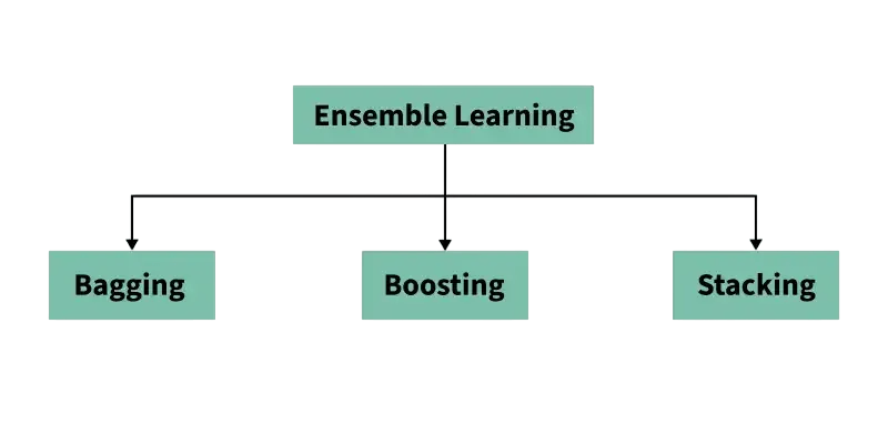
- Random Forest: An ensemble of decision trees trained on random subsets of data and features. It improves accuracy and reduces overfitting.
- Gradient Boosting: Builds trees sequentially, with each new tree correcting the errors of the previous ones. XGBoost, LightGBM, and CatBoost are popular implementations.
These ensemble techniques significantly boost the predictive power of decision trees.
Hyperparameter Tuning
To optimize decision tree performance, key hyperparameters to tune include: maximum depth, minimum samples per split, and criterion functions like Gini or entropy. To understand how these tuning strategies fit into the broader landscape, exploring What Is Machine Learning reveals how core techniques such as regression, classification, clustering, and anomaly detection empower systems to learn from data automating predictions and refining model behavior across diverse applications.
- max_depth: Maximum depth of the tree.
- min_samples_split: Minimum samples required to split a node.
- min_samples_leaf: Minimum samples required at a leaf node.
- max_features: Number of features to consider when looking for the best split.
Using tools like GridSearchCV or RandomizedSearchCV helps find the best combination of these parameters.
- from sklearn.model_selection import GridSearchCV
- params = {
- ‘max_depth’: [3, 5, 10],
- ‘min_samples_split’: [2, 5, 10]
- grid_search = GridSearchCV(DecisionTreeClassifier(), param_grid=params, cv=5)
- grid_search.fit(X_train, y_train)
- print(grid_search.best_params_)
Summary
Decision Trees are a foundational machine learning technique, known for their simplicity and interpretability.While they may not always provide the best accuracy compared to other models, they are invaluable for understanding data relationships and are frequently used in ensemble methods topics thoroughly explored in Machine Learning Training, where learners examine model interpretability, bias-variance tradeoffs, and the strategic use of weak learners in boosting and bagging frameworks. From industry applications to academic study, decision trees remain a core tool in any data scientist’s toolkit. Their role in powering more complex models like Random Forest and Gradient Boosting further cements their importance in the machine learning landscape.