Last updated on 06th Aug 2025| 11915
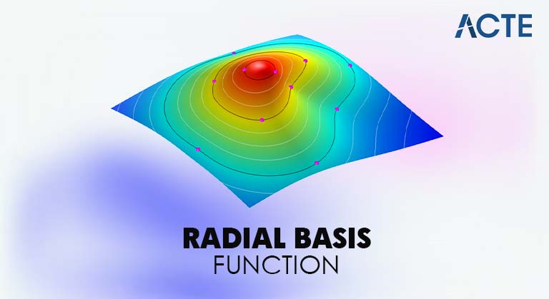
- Introduction to RBF
- Mathematical Formulation
- RBF vs Other Kernels
- RBF Networks in Machine Learning
- Hidden Layer and Gaussian Functions
- Training an RBF Network
- Applications in Classification
- Time Series and Function Approximation
- Hyperparameter Tuning in RBF
- Case Studies with RBF
- Conclusion
Introduction to RBF
Radial Basis Functions (RBFs) are a fundamental concept in machine learning and numerical analysis. Originally introduced in the context of multivariate interpolation in scattered data approximation by experts like Hardy, Micchelli, and Powell during the late 1970s, RBFs have now become cornerstones in modern predictive modeling. An RBF is a real-valued function whose output depends solely on the distance between the input and a center (prototype), not on the direction of that difference an important concept often emphasized during Machine Learning Training. This isotropic property (uniform in all directions) makes RBFs powerful tools for forming local approximations in high-dimensional spaces.
Why are RBFs important? They provide a flexible basis for approximating continuous functions. By centering multiple radial functions (commonly Gaussian) at various points in the input space and combining them linearly, one can approximate almost any nonlinear function given sufficient capacity. This forms the foundation of RBF networks three-layer neural architectures where the middle hidden layer consists of radial units centered at data-driven points. Academically and practically, RBFs strike a balance between interpretability and flexibility; they’re easier to understand than deep neural nets yet more expressive than pure linear models.
Ready to Get Certified in Machine Learning? Explore the Program Now Machine Learning Online Training Offered By ACTE Right Now!
Mathematical Formulation
At its core, an RBF is expressed as:
- ϕ(x,c)=ϕ(∥x−c∥)\phi(x, c) = \phi(\|x – c\|)ϕ(x,c)=ϕ(∥x−c∥)
- A widely used variant, Gaussian RBF, is defined as:
- ϕ(x,c)=exp(−β∥x−c∥2)\phi(x, c) = \exp\left(-\beta \|x – c\|^2\right)ϕ(x,c)=exp(−β∥x−c∥2)
Where:
- ∥x−c∥² denotes Euclidean distance squared,
- β controls the spread (width) of the Gaussian
- Sometimes expressed via σ with β = 1 / (2σ²).
Other variants include:
- Multiquadric: ∥x−c∥2+a2\sqrt{\|x – c\|^2 + a^2}∥x−c∥2+a2
- Inverse multiquadric: 1/∥x−c∥2+a21 / \sqrt{\|x – c\|^2 + a^2}1/∥x−c∥2+a2
- Thin‑plate spline: ∥x−c∥2log(∥x−c∥)\|x – c\|^2 \log(\|x – c\|)∥x−c∥2log(∥x−c∥)
But Gaussian remains the most popular for its simplicity, smoothness, and universality as a positive-definite kernel, crucial for SVM formulations and others.
RBF vs Other Kernels
RBF is often compared against polynomial and sigmoid kernels, especially within Support Vector Machine (SVM) literature an area frequently explored in What Is Machine Learning techniques.
- Expressive power: RBF kernels are universal, capable of approximating any continuous function on a compact domain. In contrast, low-degree polynomials lack flexibility, and higher-degree polynomials may overfit.
- Locality and smoothness: Gaussian RBFs emphasize local similarity, whereas polynomial kernels consider global feature interactions, which can amplify noise.
- Hyper-parameter sensitivity: RBFs need tuning of β (or γ = β) and regularization (C in SVM), making cross-validation indispensable. However, once tuned, they often deliver competitive accuracy.
- Practicality: RBFs generally outperform polynomial or sigmoid kernels in real-world classification tasks due to adaptability. Yet, RBFs are computationally more expensive, and scaling to large datasets often requires approximation techniques like Random Fourier Features or Nyström methods.
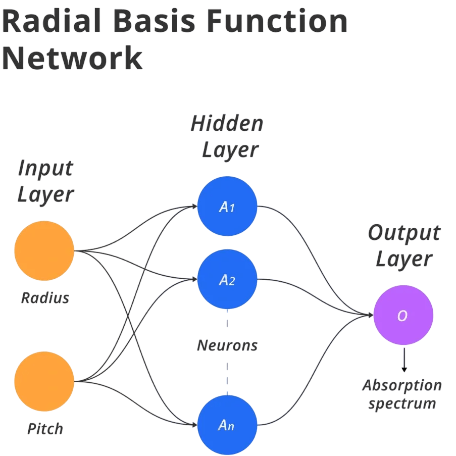
- Input Layer: Accepts raw input features x ∈ ℝd.
- Hidden Layer: C Contains N RBF units, each computing: hi(x)=exp(−β∥x−ci∥2)h_i(x) = \exp\left(-\beta \|x – c_i\|^2\right)hi(x)=exp(−β∥x−ci∥2) where cic_ici is the center (learned or pre-selected).
- Output Layer: Computes a weighted sum: y(x)=∑i=1Nwi⋅hi(x)y(x) = \sum_{i=1}^N w_i \cdot h_i(x)y(x)=i=1∑Nwi⋅hi(x) Optionally, an activation (e.g., softmax) is applied for classification.
- Face recognition: Gaussian activations detect feature clusters.
- Handwritten digit recognition: Local prototypes capture digit shapes.
- Medical diagnosis: Soft clustering of physiological data.
- Text classification: Embeddings passed through Gaussian kernels.
- Interpolation: Smoothly fill missing data points in high-dimensional spaces.
- Control systems: Approximate nonlinear plant models or control policies.
- Forecasting: Predict future values based on radial patterns.
- Anomaly detection: Learn normal patterns and flag deviations.
- Number of RBF units (N): More units increase representational capacity but also risk overfitting and memory issues.
- Center selection method: K-means clustering often yields efficient prototypes; random selection is simpler.
- Network width (σ or β): Critical for smoothness; tuned via validation.
- Regularization λ: Controls weight magnitude to avoid overfitting.
- Kernel parameters in SVM: C and γ require joint tuning.
- Medical Diagnosis (Breast Cancer Detection): RBF-ELM ensemble (Extreme Learning Machine with RBF features) achieved 97%+ accuracy on the Wisconsin dataset outperforming linear SVM baselines and highlighting RBF utility in low-dim, high-importance applications.
- RBF-SVM Benchmark on UCI Datasets: Studies across 115 binary classification problems show RBF-SVM consistently in the top tier. Bayesian-optimized parameters beat or match grid-search alternatives, underlining robust methodology.
- Weaker Performance: Users on platforms like Reddit report poor accuracy (~85–90%) using standard RBF-SVM on MNIST without PCA or advanced preprocessing, highlighting the need for dimensionality reduction and scaling in high-dimensional tasks.
- Robotic Control: RBF networks successfully model dynamic nonlinear systems (robot arms), enabling real‑time adaptive control showcasing RBFs in engineering applications.
To Explore Machine Learning in Depth, Check Out Our Comprehensive Machine Learning Online Training To Gain Insights From Our Experts!
RBF Networks in Machine Learning
An RBF network is a three-layer feedforward neural network:
Unlike traditional neural networks, RBF networks are radial basis function approximators: the hidden layer transforms inputs into localized features, and the output layer linearly combines those for prediction. This structure lends itself to closed-form training of output weights via linear methods, making RBF networks fast and interpretable.

Hidden Layer and Gaussian Functions
The hidden layer is the main part of Radial Basis Function (RBF) networks. Each hidden node works with high accuracy. These nodes focus around a specific point and use a Gaussian kernel that creates the strongest activations when inputs are close to that center a behavior that contrasts with ensemble strategies like Bagging vs Boosting in Machine Learning, where model diversity and weighting play a central role. Researchers use different strategies to choose centers. They might randomly sample from training data, use K-means clustering to find representative points, or apply advanced supervised methods that improve centers and widths through gradient descent. The width parameter (σ) plays a key role in how much area the node’s activation covers. Smaller values lead to very localized responses that can detect subtle differences but may also cause overfitting. Larger values give smoother, more general responses. When you look at these activation surfaces, each RBF appears as a smooth, centered bump. Together, they create a global function that allows for detailed and flexible machine learning representations.
Training an RBF Network
Researchers train Radial Basis Function (RBF) networks using a clear, multi-step process that ensures strong model performance. They start by selecting centers. They can do this with unsupervised methods like K-means clustering or random subsampling. They may also use supervised fine-tuning with gradient descent for better accuracy. Next, they determine the width by using heuristic methods to calculate β based on the average distances between centers or by applying cross-validation techniques to optimize σ or β over validation sets. In the key step of estimating output weights, they use linear least squares optimization a foundational technique often covered in Machine Learning Training. This solves a regularized problem that minimizes the difference between hidden activation matrices and target outputs. It also includes Ridge Regression to stabilize weights and reduce overfitting. This careful training method provides a clear advantage over deep neural networks by ensuring a global optimum through a convex problem-solving approach. This makes RBF networks an effective and dependable machine learning method.
Looking to Master Machine Learning? Discover the Machine Learning Expert Masters Program Training Course Available at ACTE Now!
Applications in Classification
In classification tasks, RBF networks serve as powerful pattern recognizers offering a contrasting approach to decision Trees in Machine Learning, which rely on recursive partitioning of the input space.
Typically, RBF networks perform classification by learning decision boundaries in radial feature space, then applying either one-hot or one-versus-rest classification schemes. Hybrid models, such as combining RBF layers with logistic regression or SVM at the output, combine representation power with discriminative learning.
Time Series and Function Approximation
RBF networks are excellent in function approximation and time-series contexts capabilities that align well with scalable solutions discussed in the Overview of ML on AWS.
The universal approximation property of RBFs makes them suitable for capturing any continuous underlying function, given sufficient basis functions. Unlike LSTMs or CNNs, they are straightforward and computationally cheap, useful for small data applications.
Preparing for Machine Learning Job Interviews? Have a Look at Our Blog on Machine Learning Interview Questions and Answers To Ace Your Interview!
Hyperparameter Tuning in RBF
Key Hyperparameter Tuning:
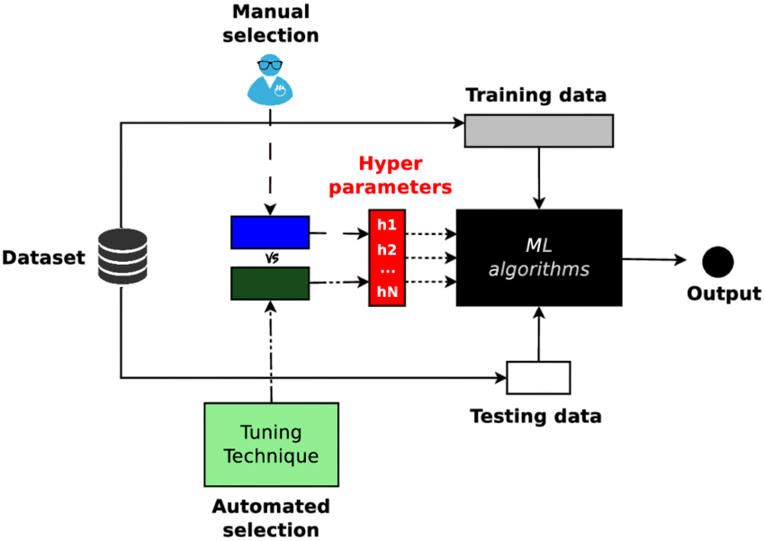
Grid search, random search, and Bayesian optimization with nested cross validation ensure Hyperparameter Tuning performance across unseen data.
Case Studies with RBF
Conclusion
Radial Basis Function (RBF) networks provide flexible solutions in many computer science areas. They are especially useful for interpolation, low-dimensional classification, engineering tasks, and quick prototyping. Researchers need to preprocess these models carefully. This involves scaling features and choosing centers wisely using techniques like K-means clustering standard practices emphasized in Machine Learning Training. Data scientists improve deployment by fine-tuning parameters. They use nested cross validation to adjust σ or γ parameters and add regularization for output weights. Although deep learning has become more popular, RBF networks still hold value with their clear, understandable structures and smooth approximation skills. Researchers can use approximate kernel methods like Random Fourier or Nyström techniques to boost performance. It’s essential to compare RBF models with simpler options to ensure the best balance of efficiency and predictive accuracy.