What is Normality Test in Minitab? – Learning Guide

Last updated on 13th Jul 2020, Blog, General

(5.0) | 17529 Ratings 1454

Share:

The one-sample t-test is used to determine whether a sample comes from a population with a specific mean. This population mean is not always known, but is sometimes hypothesized.

For example, imagine that an academic was conducting research on the relationship between exam performance and revision time, but wanted to first check whether his 100 participants reflected the national average in terms of their academic ability, measured in terms of their GMAT score. The academic could use a one-sample t-test to compare the GMAT score of the 100 participants against the national average. Alternately, imagine that a lecturer believed her course required 10 hours of study time per week and wanted to determine whether students spent this amount of time studying. The lecturer could use a one-sample t-test to compare the weekly study time of a sample of 20 students to the suggested 10 hours.

In this guide, we show you how to carry out a one-sample t-test using Minitab, as well as interpret and report the results from this test. However, before we introduce you to this procedure, you need to understand the different assumptions that your data must meet in order for a one-sample t-test to give you a valid result. We discuss these assumptions next.

A one-sample t-test has four assumptions. You cannot test the first two of these assumptions with Minitab because they relate to your study design and choice of variables. However, you should check whether your study meets these two assumptions before moving on. If these assumptions are not met, there is likely to be a different statistical test that you can use instead. Assumptions #1 and #2 are explained below:

• Assumption #1: Your dependent variable should be measured at a continuous level (i.e., it is an interval or ratio variable). Examples of continuous variables include height (measured in feet and inches), temperature (measured in °C), salary (measured in US dollars), revision time (measured in hours), intelligence (measured using IQ score), firm size (measured in terms of the number of employees), age (measured in years), reaction time (measured in milliseconds), grip strength (measured in kg), power output (measured in watts), test performance (measured from 0 to 100), sales (measured in number of transactions per month), academic achievement (measured in terms of GMAT score), and so forth. If you are unsure whether your dependent variable is continuous (i.e., measured at the interval or ratio level), see our Types of Variable guide.
• Assumption #2: The data are independent (i.e., not correlated/related), which means that there is no relationship between the observations. This is more of a study design issue than something you can test for, but it is an important assumption of the one-sample t-test.

Assumptions #3 and #4 relate to the nature of your data and can be checked using Minitab. You have to check that your data meets these assumptions because if it does not, the results you get when running a one-sample t-test might not be valid. In fact, do not be surprised if your data violates one or more of these assumptions. This is not uncommon. However, there are possible solutions to correct such violations (e.g., transforming your data) such that you can still use a one-sample t-test. Assumptions #3 and #4 are explained below:

• Assumption #3: There should be no significant outliers. An outlier is simply a case within your data set that does not follow the usual pattern. For example, consider a study examining the test anxiety of 500 students where anxiety was measured on a scale of 0-100, with 0 = no anxiety and 100 = maximum anxiety. The mean test anxiety score was 56 and the vast majority of students scored between 42 and 70. However, one student scores just 2 on the scale, with the second lowest test anxiety score being 36. As such, a student scoring just 2 on the scale “could” be considered an outlier. Where a score is an outlier this is problematic because outliers can have a disproportionately negative effect on the one-sample t-test, reducing the accuracy of its results. Fortunately, when using Minitab to run a one-sample t-test on your data, you can easily detect possible outliers.
• Assumption #4: Your dependent variable should be approximately normally distributed. We talk about the one-sample t-test only requiring approximately normal data because it is quite “robust” to violations of normality, meaning that the assumption can be a little violated and still provide valid results. You can test for normality using the Shapiro-Wilk test of normality, which is easily tested for using Minitab.

Histograms are efficient graphical methods for describing the distribution of data. It is always a good practice to plot your data in a histogram after collecting the data. This will give you an insight about the shape of the distribution and whether it is normal or not. If the data is symmetrically distributed and most results are located in the middle, we can say that the data is normally distributed.

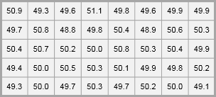
Suppose that a line manager is seeking to assess how consistently a production line is producing. He is interested in the weight of a food products with a target of 50 grams per item. He takes a random sample of 40 products and measures their weights. For this example, we may use the product_weight worksheet. Remember to copy the data from the Excel worksheet and paste it into the Minitab worksheet.

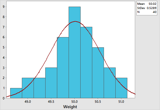
To create a histogram in Minitab, select Graph > Histogram > With Fit, specify the column of data to analyze, in this case ‘product weight’, and then click OK. The figure below shows a histogram which suggests that the data is normally distribution. Notice how the data is symmetrically distributed and concentrated in the center of the histogram.

We can also construct a Normal Probability Plot to test the assumption of normality. This provides a more decisive approach for deciding if a data set is normally distributed. All points for a normal distribution should approximately form a straight line that falls between 95% confidence interval limits.

To create a normal probability plot in Minitab, select Graph > Probability Plot > Single, specify the column of data to analyze, leave the distribution option to be normal, and then click OK. Here is a screenshot of the example result for our previous product_weight example:

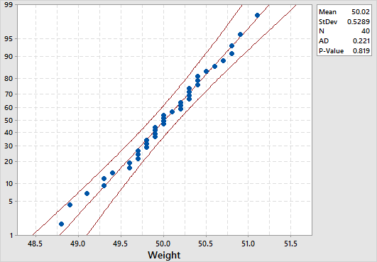
The normal distribution is a good fit if the data points approximately follow a straight line. In our example, the data points approximately follow a straight line that falls mainly between the 95% confidence interval limits, and so it can be concluded that the data is normally distributed.

The Anderson-Darling Normality Test measures how well the data follow the normal distribution (or any particular distribution). It is a statistical test that compares the actual distribution with the theoretical normal distribution. A lower p-value than the significance level (normally 0.05) indicates a lack of normality in the data (regardless of the AD value). Remember to keep your eyes on the histogram and the normal probability plot in conjunction with the Anderson-Darling test before making any decision.

To conduct an Anderson-Darling normality test in Minitab, select Stat > Basic Statistics > Normality Test, specify the column of data to analyze, then specify the test method to be Anderson-Darling, and then click OK. The p-value in our product_weight example is 0.819 which suggests that the data follow the normal distribution. Note that both the graphical summary and the probability plot displays Anderson-Darling normality test results by default.