
Last updated on 03rd Jan 2022| 1845
Dimensionality Reduction (DR) is the pre-processing step to remove redundant features, noisy and irrelevant data, in order to improve learning feature accuracy and reduce the training time.
- What is Dimensionality Reduction?
- Why is Dimensionality Reduction required?
- Common Dimensionality Reduction Techniques
- Conclusion
- Facebook assembles data of what you like, share, post, places you visit, bistros you like, etc
- Your wireless applications assemble a lot of individual information about you
- Amazon assembles data of what you buy, view, click, etc their site
- Betting clubs screen each move each customer makes
What is Dimensionality Reduction?
We are making a huge proportion of data step by step. Without a doubt, 90% of the data in the world has been made in the last 3-4 years! The numbers are truly astounding. Coming up next are just a piece of the occasions of the kind of data being accumulated:
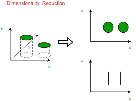
As data age and arrangement keeps growing, envisioning it and attracting enlistments ends up being progressively troublesome. Maybe the most notable method of doing discernment is through outlines. Accept we have 2 elements, Age and Height. We can use a scatter or line plot among Age and Height and envision their relationship with no issue:
By and by consider a case wherein we have, say 100 variables (p=100). For the present circumstance, we can have 100(100-1)/2 = 5000 particular plots. It doesn’t look at to imagine all of them autonomously, right? In such circumstances where we have innumerable elements, it is more intelligent to pick a subset of these variables (p<<100) which gets as much information as the main plan of elements.
- Space needed to store the information is decreased as the quantity of aspects descends
- Less aspects lead to less calculation/preparing time
- A few calculations don’t perform well when we have an enormous aspects. So lessening these aspects needs to occur for the calculation to be helpful
- It deals with multicollinearity by eliminating excess highlights. For instance, you have two factors – ‘time spent on treadmill in minutes’ and ‘calories consumed’. These factors are profoundly related as the additional time you spend running on a treadmill, the more calories you will consume. Henceforth, there is no good reason for putting away both as only one of them does what you require
- It helps in envisioning information. As examined before, it is extremely challenging to envision information in higher aspects so decreasing our space to 2D or 3D might permit us to plot and notice designs all the more obviously
Why is Dimensionality Reduction required?
Here are a portion of the advantages of applying dimensionality decrease to a dataset:

Develop Your Skills with Advanced Dimensional Data Modeling Certification Training
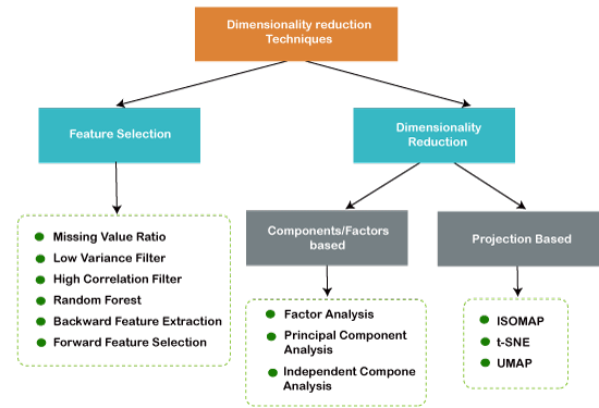
Weekday / Weekend BatchesSee Batch Details- Missing Value Ratio
- Low Variance Filter
- High Correlation Filter
- Random Forest
- Backward Feature Elimination
- Forward Feature Selection
- Factor Analysis
- Principal Component Analysis
- Independent Component Analysis
- UMAP
- We first take all the n factors present in our dataset and train the model utilizing them
- We then, at that point, work out the presentation of the model
- Presently, we process the exhibition of the model subsequent to wiping out every factor (n times), i.e., we drop one variable without fail and prepare the model on the excess n-1 factors
- We distinguish the variable whose evacuation has created the littlest (or no) adjustment of the presentation of the model, and afterward drop that variable
- Rehash this cycle until no factor can be dropped
- We start with a solitary component. Basically, we train the model n number of times utilizing each element independently
- The variable giving the best exhibition is chosen as the beginning variable
- Then, at that point, we rehash this cycle and add each factor in turn. The variable that creates the most elevated expansion in execution is held
- We rehash this cycle until no huge improvement is found in the model’s presentation
- A key part is a direct mix of the first factors
- Head parts are extricated so that the primary head part clarifies most extreme change in the dataset
- Second head part attempts to clarify the excess change in the dataset and is uncorrelated to the primary head part
- Third head part attempts to clarify the difference which isn’t clarified by the initial two head parts, etc.
Common Dimensionality Reduction Techniques:
Missing Value Ratio
Assume you’re given a dataset. What might be your initial step? You would normally need to investigate the information first prior to building model. While investigating the information, you find that your dataset makes them miss esteems. What’s the deal? You will attempt to discover the justification behind these missing qualities and afterward ascribe them or drop the factors altogether which have missing qualities (utilizing suitable strategies).
Low Variance Filter
Consider a variable in our dataset where every one of the perceptions have a similar worth, say 1. In the event that we utilize this variable, do you figure it can further develop the model we will fabricate? The response is no, in light of the fact that this variable will have zero change.
Along these lines, we want to work out the change of every factor we are given. Then, at that point, drop the factors having low change when contrasted with different factors in our dataset. The justification behind doing this, as I referenced above, is that factors with a low change won’t influence the objective variable.
High Correlation Filter
High relationship between’s two factors implies they have comparable patterns and are probably going to convey comparable data. This can cut down the presentation of certain models radically (direct and calculated relapse models, for example). We can compute the connection between’s free mathematical factors that are mathematical in nature. On the off chance that the relationship coefficient passes a specific boundary esteem, we can drop one of the factors (dropping a variable is exceptionally emotional and ought to forever be finished remembering the area).
Random Forest
Arbitrary Forest is one of the most generally involved calculations for highlight determination. It comes bundled with in-fabricated component significance so you don’t have to program that independently. This assists us with choosing a more modest subset of highlights.
We really want to change over the information into numeric structure by applying one hot encoding, as Random Forest (Scikit-Learn Implementation) takes just numeric data sources. How about we likewise drop the ID factors (Item_Identifier and Outlet_Identifier) as these are simply remarkable numbers and hold no huge significance for us as of now.
Backward Feature Elimination
Follow the underneath steps to comprehend and utilize the ‘Retrogressive Feature Elimination’ strategy:
Forward Feature Selection
This is the contrary course of the Backward Feature Elimination we saw previously. Rather than killing highlights, we attempt to observe the best elements which work on the exhibition of the model. This strategy functions as follows:
Factor Analysis
Assume we have two factors: Income and Education. These factors will conceivably have a high connection as individuals with an advanced education level will generally have essentially higher pay, as well as the other way around.
In the Factor Analysis method, factors are assembled by their connections, i.e., all factors in a specific gathering will have a high relationship among themselves, yet a low relationship with factors of other group(s). Here, each gathering is known as a variable. These variables are little in number when contrasted with the first elements of the information. Nonetheless, these elements are hard to notice.
Principal Component Analysis
PCA is a procedure which helps us in separating another arrangement of factors from a current huge arrangement of factors. These recently removed factors are called Principal Components. You can allude to this article to find out about PCA. For your speedy reference, beneath are a portion of the central issues you should be aware of PCA prior to continuing further:
Independent Component Analysis
Independent Component Analysis (ICA) depends on data hypothesis and is likewise perhaps the most broadly utilized dimensionality decrease technique. The significant distinction among PCA and ICA is that PCA searches for uncorrelated variables while ICA searches for autonomous elements.
On the off chance that two factors are uncorrelated, it implies there is no direct connection between them. Assuming they are autonomous, it implies they are not subject to different factors. For instance, the age of an individual is autonomous of what that individual eats, or how much TV he/she watches.
UMAP
t-SNE functions admirably on huge datasets yet it additionally has it’s constraints, for example, loss of huge scope data, slow calculation time, and failure to genuinely address exceptionally enormous datasets. Uniform Manifold Approximation and Projection (UMAP) is an aspect decrease strategy that can save as a large part of the neighborhood, and a greater amount of the worldwide information structure when contrasted with t-SNE, with a more limited runtime.
Conclusion:-
This is as exhaustive an article on dimensionality decrease as you’ll find anyplace! I had loads of fun composing it and observed a couple of better approaches for managing big number of factors I hadn’t utilized previously (like UMAP).
Managing thousands and millions of elements is an absolute necessity have ability for any information researcher. How much information we are producing every day is uncommon and we want to track down various ways of sorting out some way to utilize it. Dimensionality decrease is an extremely helpful method for doing this and has done some amazing things for me, both in an expert setting just as in AI hackathons.