Last updated on 08th Aug 2025| 12907
- Introduction to Bayes Theorem
- Mathematical Explanation
- Conditional Probability
- Naive Bayes Classifier
- Assumptions and Limitations
- Bayesian Networks
- Spam Detection with Bayes
- Parameter Estimation
- Conclusion
Introduction to Bayes Theorem
Bayes Theorem in Machine Learning is a fundamental concept in probability theory and statistics that allows us to update the probability of a hypothesis based on new evidence. Named after Thomas Bayes, it forms the foundation for a wide range of applications in machine learning, especially in classification and probabilistic reasoning. Bayesian thinking contrasts with frequentist approaches by allowing for the incorporation of prior beliefs. This makes it particularly useful in real-world scenarios where data is uncertain, incomplete, or dynamic. In artificial intelligence (AI) and Machine Learning Training (ML), Bayes Theorem is the core behind models such as the Naive Bayes classifier, Bayesian networks, and even Bayesian deep learning.Bayes’ Theorem is a fundamental concept in probability theory and statistics that describes how to update the probability of a hypothesis based on new evidence. Named after the mathematician Thomas Bayes, the theorem provides a mathematical framework for reasoning under uncertainty. It is widely used in fields such as machine learning, data science, medicine, finance, and artificial intelligence.
Ready to Get Certified in Machine Learning? Explore the Program Now Machine Learning Online Training Offered By ACTE Right Now!
Mathematical Explanation
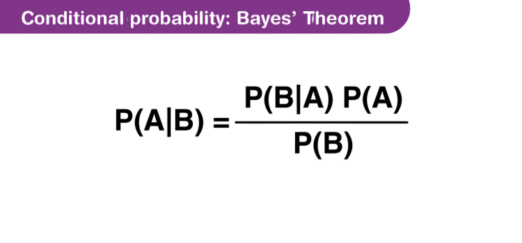
Bayes Theorem is stated as:
P(A∣B)=P(B∣A)⋅P(A)P(B)P(A|B) = \frac{P(B|A) \cdot P(A)}{P(B)}
Where:
- P(A∣B)P(A|B): Posterior probability – the probability of event A occurring given that B is true.
- P(B∣A)P(B|A): Likelihood – the probability of B given A.
- P(A)P(A): Prior probability – the initial belief about A.
- P(B)P(B): Marginal likelihood – the probability of B under all possible hypotheses.
Example
Suppose you’re testing for a rare disease:
- Disease prevalence (prior): P(Disease)=0.01P(Disease) = 0.01
- Test sensitivity: P(Positive∣Disease)=0.99P(Positive | Disease) = 0.99
- Test false positive rate: P(Positive∣NoDisease)=0.05P(Positive | No Disease) = 0.05
Using Bayes Theorem in Machine Learning , What is Perceptron & Tutorial you can compute the actual chance of having the disease if the test is positive.This insight is critical in fields such as medical diagnostics, spam detection, and NLP, where decisions rely on probabilistic inference.
Conditional Probability
Conditional probability is the probability of one event occurring given that another event has already occurred. It’s written as:
What Is Artificial Neural Networks This concept underpins Bayes Theorem, as it allows us to revise beliefs based on new data.
Real-world Example:
You’re told that someone likes chess. What’s the probability they’re a math teacher? This depends on how common math teachers are and how likely math teachers are to like chess. Conditional probability allows models to make context-sensitive predictions a key requirement in natural language understanding, recommendation engines, and fraud detection.
To Explore Machine Learning in Depth, Check Out Our Comprehensive Machine Learning Online Training To Gain Insights From Our Experts!
Naive Bayes Classifier
Naive Bayes is a family of simple probabilistic classifiers based on applying Bayes Theorem with a naive independence assumption: Cyber Extortion features are conditionally independent given the class. Despite this simplification, Naive Bayes often performs surprisingly well in practice.
Types of Naive Bayes Classifiers:
- Gaussian Naive Bayes: Assumes features follow a normal distribution.
- Multinomial Naive Bayes: Suitable for document classification with word counts.
- Bernoulli Naive Bayes: Works with binary features (e.g., presence or absence of a word).
Example: Spam Classification
Given an email with certain words, you calculate:
P(Spam∣Words)∝P(Words∣Spam)⋅P(Spam)P(Spam|Words) \propto P(Words|Spam) \cdot P(Spam)
Using the word probabilities conditioned on spam/non-spam training data, the model classifies new emails.

Assumptions and Limitations
Assumptions:
- Feature Independence: Naive Bayes assumes all features are independent given the label, which rarely holds true in real life.
- Feature Relevance: It assumes every feature contributes equally to the prediction.
- Data Sufficiency: Needs sufficient data to estimate class-conditional probabilities accurately.
Limitations:
- Poor performance when features are highly correlated (e.g., in image recognition).
- Artificial Intelligence and Machine Learning Tends to perform worse than more complex models like Random Forest or XGBoost on structured data.
- Sensitive to imbalanced datasets.
Yet, its efficiency and robustness on text-based tasks make it a go-to algorithm in many NLP and filtering applications.
Looking to Master Machine Learning? Discover the Machine Learning Expert Masters Program Training Course Available at ACTE Now!
Bayesian Networks
Bayesian Networks are graphical models that represent the probabilistic relationships among a set of variables using a Directed Acyclic Graph (DAG).Each node represents a random variable, and the edges represent conditional dependencies.Bayesian Networks, also known as Belief Networks or Probabilistic Graphical Models, Bayes Theorem in Machine Learning Training are powerful tools that represent probabilistic relationships among a set of variables. They combine principles from probability theory and graph theory to model complex systems with uncertainty in a structured way.
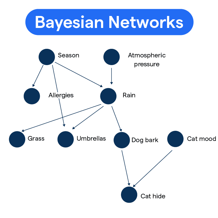
A Bayesian Network is a directed acyclic graph (DAG) where:
- Nodes represent random variables (which can be observable data, unknown parameters, or hypotheses).
- Edges represent conditional dependencies between these variables.
Each node is associated with a conditional probability distribution (CPD) that quantifies the effect of the parent nodes on the node. If a node has no parents, its CPD reduces to a prior probability. Bayesian Networks enable efficient computation of joint and conditional probabilities by exploiting the conditional independencies encoded in the graph structure. They are widely used in various fields such as medical diagnosis, risk assessment, machine learning, and decision-making systems, Parameter Estimation where reasoning under uncertainty is crucial. By incorporating evidence (observed data), Bayesian Networks can update the probabilities of unknown variables using Bayes’ Theorem, making them excellent for inference and prediction in complex domains.Bayesian networks can perform exact and approximate inference and are used in advanced probabilistic systems, including recommendation engines and decision support systems.
Spam Detection with Bayes
Spam Detection with Bayes is one of the earliest and most successful applications of Naive Bayes.Spam Detection with Bayes is a classic application of Bayesian methods, particularly using the Naive Bayes classifier, which applies Bayes’ Theorem with the assumption that features (such as words in an email) are independent given the class (spam or not spam). Computer Vision & How does it Works In this approach, each email is represented by features extracted from its content commonly the presence or frequency of certain words. The goal is to calculate the probability that an email is spam based on these features. Using Bayes’ Theorem, the probability that an email is spam given the words it contains is:
p(Spam∣Words)=P(Words∣Spam)×P(Spam)P(Words)P(\text{Spam} | \text{Words}) = \frac{P(\text{Words} | \text{Spam}) \times P(\text{Spam})}{P(\text{Words})}P(Spam∣Words)=P(Words)P(Words∣Spam)×P(Spam)
The Naive Bayes assumption simplifies computation by treating the presence of each word as independent, so:
P(Words∣Spam)=∏iP(Wordi∣Spam)P(\text{Words} | \text{Spam}) = \prod_{i} P(\text{Word}_i | \text{Spam})P(Words∣Spam)=i∏P(Wordi∣Spam)
The classifier calculates this probability for both “Spam” and “Not Spam” classes and assigns the label with the higher probability. This method is popular because it is simple, fast, and often surprisingly effective, even with the strong independence assumption. It adapts well to new spam patterns by updating word probabilities as more labeled emails are processed.
Workflow:
- Collect Data: Use labeled email datasets (e.g., SpamAssassin).
- Preprocessing: Tokenization, stop-word removal, stemming.
- Feature Extraction: Term frequency, TF-IDF, or binary presence.
- Train Naive Bayes using labeled data.
- Predict whether new emails are spam.
Preparing for Machine Learning Job Interviews? Have a Look at Our Blog on Machine Learning Interview Questions and Answers To Ace Your Interview!
Parameter Estimation
An Overview of ML on AWS Parameter estimation in Bayesian inference refers to estimating the posterior distribution of model parameters.
Two primary methods:
- Maximum Likelihood Estimation (MLE): Finds parameters that maximize the likelihood of the observed data.
- Maximum A Posteriori (MAP): Maximizes the posterior distribution, combining likelihood and prior beliefs.
- MLE estimates P(word∣class)P(word|class) from frequency.
- MAP adds Laplace smoothing to prevent zero probabilities.
Formula:
MAP(θ)=argmaxθP(θ∣X)∝P(X∣θ)⋅P(θ)MAP(\theta) = \arg \max_\theta P(\theta|X) \propto P(X|\theta) \cdot P(\theta)
In Naive Bayes:
Summary
Bayes Theorem in Machine Learning is a powerful statistical tool that allows intelligent systems to reason under uncertainty. Its applications in Machine Learning Training , particularly through Naive Bayes and Bayesian networks, make it indispensable for tasks ranging from spam filtering to medical diagnostics.Spam detection uses Bayes’ Theorem to classify emails as Spam Detection with Bayes or not based on the words they contain. The Naive Bayes classifier assumes word independence, calculating the probability that an email is spam given its words. It compares this against the probability of the email being legitimate and labels it accordingly. This approach is simple, fast, and effective, Parameter Estimation making it widely used in filtering unwanted emails.